How to Freeze Title Row in Excel (Easiest Way in 2024)

In this article, we will show you how to the freeze title row in Excel. Simply follow the steps below.

How to Freeze Titles in Excel

To freeze the title row in Excel, simply select the row below titles and choose “Freeze Top Row” under the View tab. Here’s how to do it:

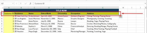
1. Identify the Title Row you Want to Freeze

Scroll through your spreadsheet and find the row containing the titles or headers you want to freeze. This is typically the first row.

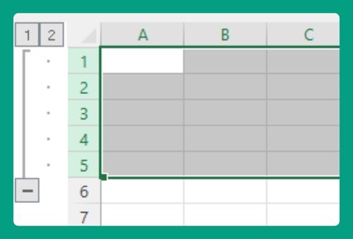
2. Select the Row Below the Title Row

Click on the row number of the row directly below the title row. For example, if your title row is row 1, click on the number for row 2 to select it.

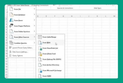
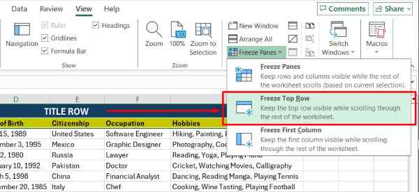
3. Go to the “View” tab to Freeze Title Row

Look at the top of the Excel window and locate the ribbon menu. Click on the “View” tab to access the view options. In the “Window” group of the View tab, find the “Freeze Panes” dropdown menu. Click on it to reveal the options.

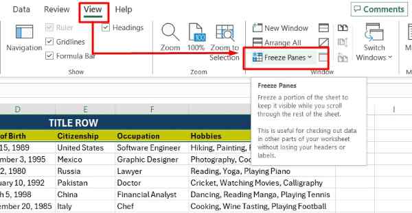
4. Select “Freeze Top Row” from the Dropdown Menu

From the dropdown menu, choose “Freeze Top Row.” This will freeze the selected row (row 2) and keep it visible at the top of the spreadsheet, even when scrolling down.

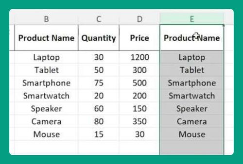
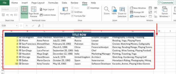
5. Verify if the Title Row is Frozen

Scroll through your spreadsheet to ensure that the title row remains visible at the top, even as you navigate through the rest of the data. You should be able to scroll down without losing sight of the titles.

We hope you now better understand how to freeze the title row in Excel. If you enjoyed this article, you might also like our article on How to Unfreeze Panes in Excel or our article on How to Freeze Header in Excel.