How to Freeze Specific Columns in Excel (Easiest Way in 2024)

In this article, we will show you how to freeze specific columns in Excel. Simply follow the steps below.

How to Freeze Selected Columns in Excel

Follow the steps below to easily freeze selected columns in Excel.

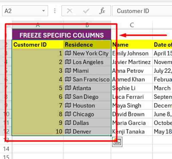
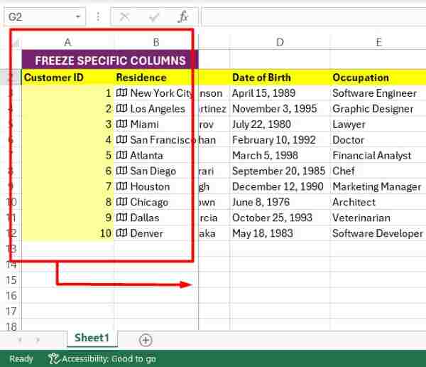
1. Select the Specific Columns You Want to Freeze

Scroll horizontally to find the columns you want to remain visible while you work with your data. Then, select the columns you want to freeze.

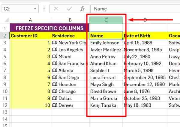
2. Click on the Column to the Right

To freeze the selected columns, start by locating the column header that follows the last column you intend to freeze. For example, if you aim to freeze columns A and B, click on the column header for column C. This action ensures that the columns to the left of the selected column header remain visible.

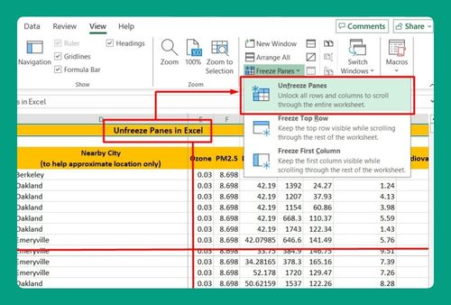
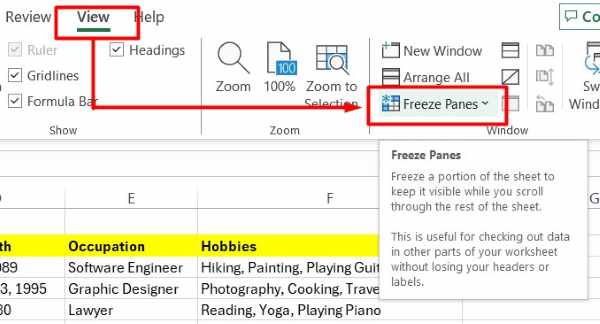
3. Access the “View” Tab on the Excel Ribbon

Go to the “View” tab located at the top of Excel. This tab contains various viewing options to customize your Excel experience. Then, look for the “Window” group. Click on “Freeze Panes” to lock the chosen columns in place.

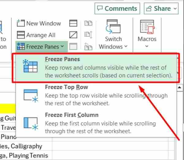
4. Select “Freeze Panes” from the Dropdown Menu

A dropdown menu will appear after clicking on “Freeze Panes.” Choose the “Freeze Panes” option from this menu to freeze the selected columns effectively. This action ensures that the chosen columns remain fixed in their positions.

5. Confirm the Freezing of Selected Columns

After selecting “Freeze Panes,” verify that the chosen columns remain visible while you scroll horizontally and vertically. This confirms that your desired columns are successfully frozen.

We hope you now better understand how to freeze specific columns in Excel. If you enjoyed this article, you might also like our article on how to freeze specific rows in Excel or our article on how to freeze formula in Excel.