How to Split a Cell Diagonally in Excel (Easiest Way in 2025)
In this article, we will explore how to split cells diagonally in Excel by creating diagonal borders. Simply follow the steps below.
How to Split Cells Diagonally in Excel
Follow the steps below to split cells diagonally in Excel by creating diagonal borders.
1. Enter the Data
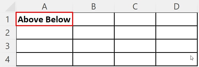
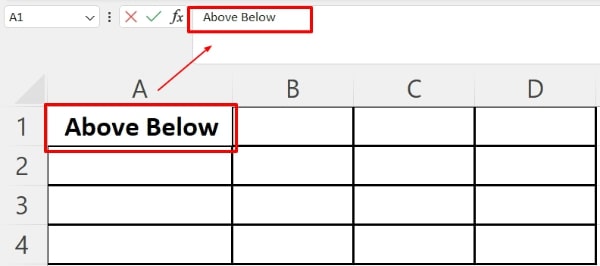
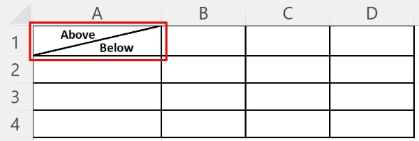
Select the cell where you want to split diagonally and enter the two words you want to split. For this example, we will use “Above” and “Below”. Initially enter them as “Above Below”.
2. Open the “Format Cells” Dialog Box
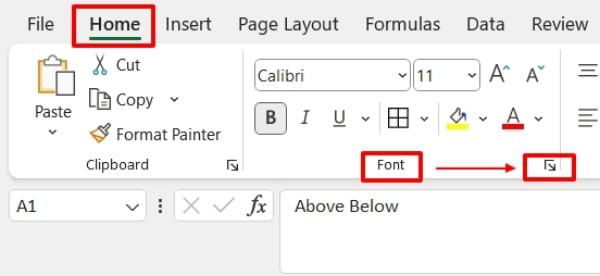
Click on the cell and go to the “Home” tab on the Ribbon. Expand the “Font” tool group to launch the “Formal Cells” dialog box.
3. Apply a Diagonal Border
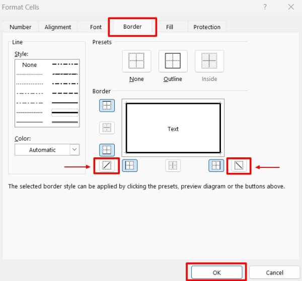
Click on the “Borders” tab and select a diagonal line style (either “Diagonal down” or “Diagonal up” depending on your preference).
4. Confirm the Formatting
Click “OK” to apply the diagonal border.

5. Adjust the Text Alignment
Select the cell and highlight the first word (“Above”) from the formula bar.
6. Format the First Word as Superscript
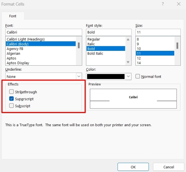
While the first word is still highlighted, open the “Format Cells” dialog box again from the “Font” tool group. Select “Superscript” under “Effects”. This will set the first word above the diagonal border.
7. Format the Second Word as Subscript
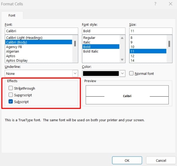
Go back to the cell and highlight the second word (“Below”) from the formula bar. Access the “Format Cells” dialog box again and select “Subscript”. This will set the second word below the diagonal border.
8. Apply and Exit
Click “OK” to close the dialog box. This visually splits the cell into two diagonal sections, with one word above and one word below the diagonal border.
We hope that you now have a better understanding of how to split cells diagonally in Excel. If you enjoyed this article, you might also like our article on how to split cells horizontally in excel and how to remove split screen in excel.

