How to Add Multiple Trendlines in Excel (2024 Guide)

In this article, we will show you how to add multiple trendlines in Excel. Simply follow the steps below!

Add Multiple Trendlines in Excel

Below we explain the step by step process on how to add multiple trendlines in Excel:

1. Prepare Your Data

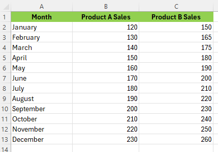
First, ensure your data is organized. For example, let’s say you have monthly sales data for two different products over one year. Organize your data in three columns: Month, Product A Sales, and Product B Sales.

2. Insert a Chart

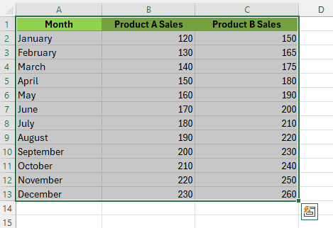
Select your data including the headers.

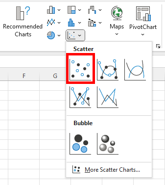
Go to the Insert tab.

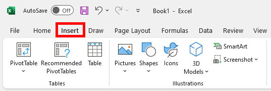
Click on Chart and choose the standard Scatter Chart.

3. Add a Trendline to the First Data Series

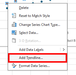
Click on one of the data points for Product A in the chart. Right-click and select Add Trendline.

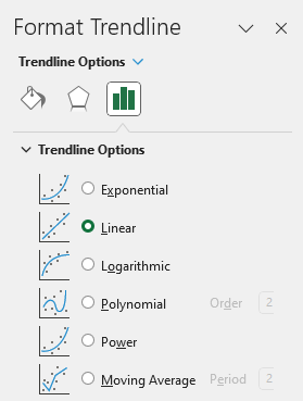
In the Format Trendline pane on the right, choose the type of trendline you want (linear, exponential, etc.). Customize the trendline’s color and style if desired.

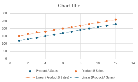
Do the same for Product B and the rest of your data points.

Here’s what our example looks like:

We hope that you now have a better understanding of how to add multiple trendlines in Excel. If you enjoyed this article, you might also like our articles on how to get rid of blank lines in Excel and how to add trendlines in Excel.