How to Add Column Sparklines in Excel (2024 Update)

In this article, we will show you how to add column sparklines in Excel. Simply follow the steps below!

How to Insert Column Sparklines in Excel

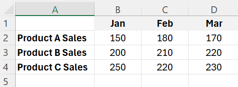
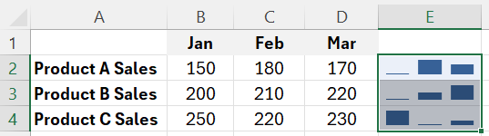
Follow the process below to add column sparklines in Excel. Here’s our sample dataset:

1. Select the Cell for Sparkline

Click on the cell where you want the sparkline to appear. Typically, this would be next to your data; for instance, select E2.

2. Insert Sparkline

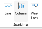
Go to the Insert tab on the Ribbon.

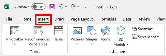
Click on the Sparklines group and choose Column.

Excel will open a “Create Sparklines” dialog box.

3. Specify Data Range

In the dialog box, for “Data Range”, select the range of data you want to include in the sparkline. In our example, select B2:D2. For “Location Range”, make sure it includes E2.

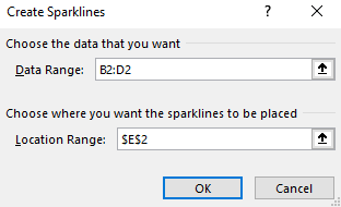
After setting the data range, click “OK”. Excel will create the sparkline in E2.

4. Copy Sparkline to Other Cells

With E2 selected, drag the fill handle (a small square at the bottom-right corner of the cell) down through E4 to copy the sparkline to each row.

We hope that you now have a better understanding of how to add column sparklines in Excel. If you enjoyed this article, you might also like our articles on how to create trend lines in Excel and how to add vertical lines to an Excel chart.