Highlight Selected Row in Excel (Easiest Way in 2025)
In this article, we will show you how to highlight an entire row in Excel when a cell is selected. Simply follow the steps below.
How to Highlight Selected Row in Excel
To highlight selected row in Excel, we will use a dataset that contains the shoe brand in Column A, their models in Column B, and the prices in Column C. Follow the steps below:
1. Select the Entire Row by Clicking the Row Number
Click the row number on the left side to select the entire row you want to highlight. For example, to select the row with the Nike Air Max 270, click on row number 2.

2. Open the Conditional Formatting Menu
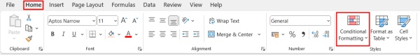
In the Home tab, find the Conditional Formatting option in the Styles group. Click on it to open the menu. This menu allows you to create rules that automatically format cells based on their values or formulas.
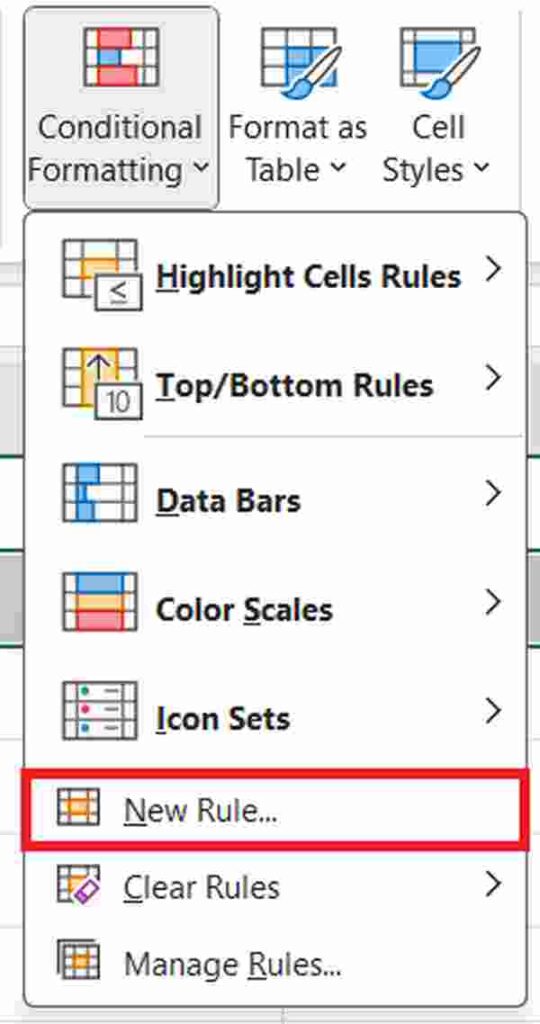
3. Select the New Rule Option
From the Conditional Formatting menu, select the “New Rule” option. This will open the New Formatting Rule dialog box, where you can define a new rule for formatting.
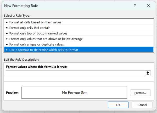
4. Select the Option to Use a Formula to Determine Formatting
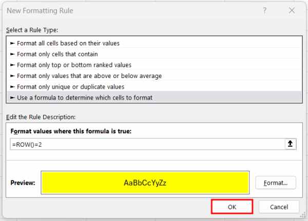
In the New Formatting Rule dialog box, select the option “Use a formula to determine which cells to format.” This option allows you to create a custom rule based on a formula that you specify.
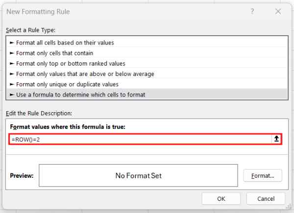
5. Enter the Formula to Highlight the Row
In the formula field, enter `=ROW()=selected_row_number,’ replacing `selected_row_number` with the number of the row you want to highlight.
For instance, to highlight the row with the Nike Air Max 270, enter `=ROW()=2`. This formula checks if the current row matches the specified row number.
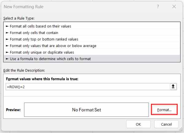
6. Click Format to Choose Highlighting Options
Click the Format button to open the Format Cells dialog box.
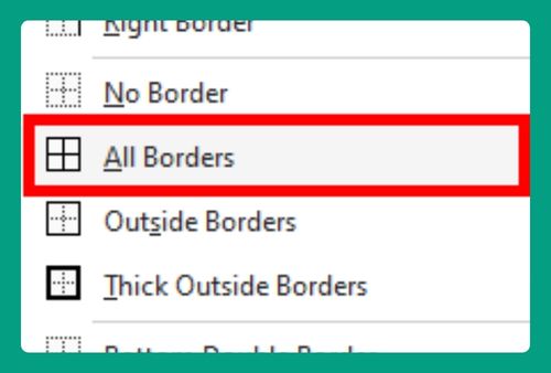
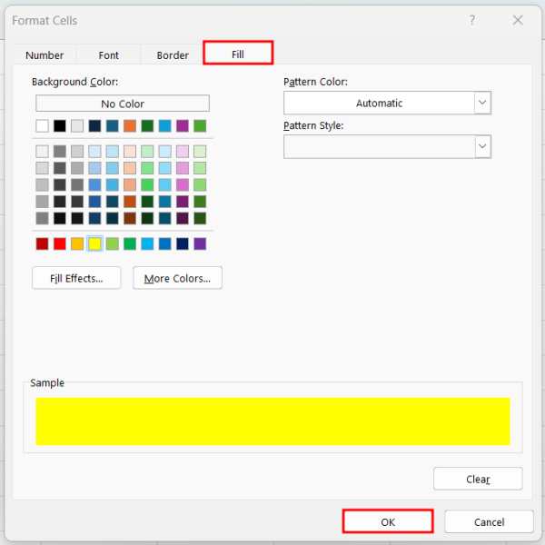
Here, you can choose the formatting options you want for the highlighted row, such as background color, font color, and border styles. In our case, let’s select to Fill and select the color yellow for the highlight color. After selecting your preferred options, click OK to apply them.
7. Apply the Rule by Clicking OK
After setting the format, click OK in the New Formatting Rule dialog box to apply the rule. This will close the dialog box and apply the conditional formatting to the selected row.
8. Verify the Row is Highlighted Correctly
Check your worksheet to ensure the selected row is highlighted according to the formatting options you chose.

We hope that you now have a better understanding of how to highlight selected row in Excel. If you enjoyed this article, you might also like our article on how to highlight specific text in Excel or our article on how to compare two columns in Excel and highlight matches.