How to Put a Checkbox In Excel (Easiest Way in 2025)
In this article, we will show you how to put a checkbox in Excel. Simply follow the steps below.
Tick Box in Excel
Follow the steps below on how to put a checkbox in Excel.
1. Enable the Developer Tab in Excel
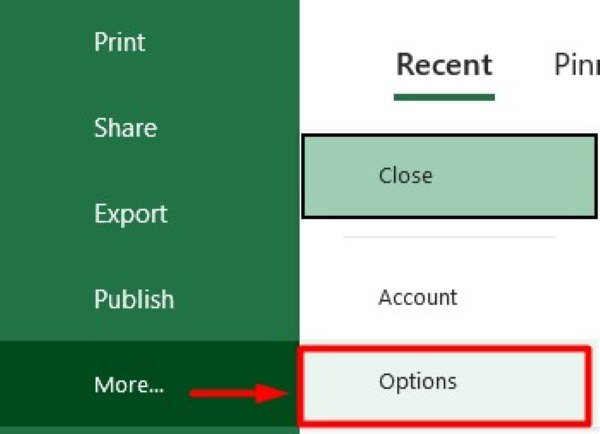
Open Excel. If the Developer tab is not visible, you need to enable it. Go to “File” at the top left corner, then select “Options”.
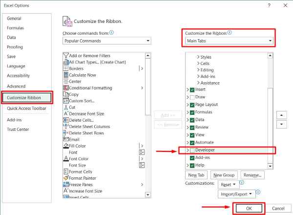
In the Excel Options window, click on “Customize Ribbon” on the left side. In the right pane, find the “Main Tabs” section and check the box next to “Developer”. Click “OK”. The Developer tab should now appear on the Excel ribbon.
2. Insert a Checkbox in Your Worksheet
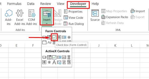
Click on the Developer tab to open its menu. In the “Controls” group, click the “Insert” button. A drop-down menu will appear. Under “Form Controls”, click the checkbox icon (it looks like a small square with a checkmark). Your cursor will change to a crosshair. Click anywhere in the worksheet where you want to place the checkbox. A checkbox will appear at the location you clicked.
3. Change the Text Label of the Checkbox
By default, the checkbox will have the label “Check Box 1”. To change this label to something more meaningful, right-click on the checkbox.
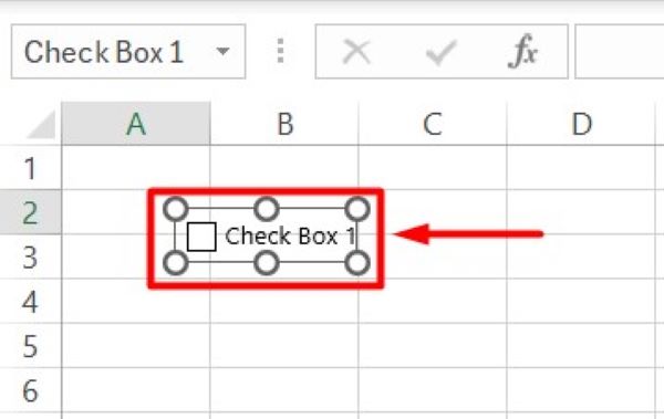
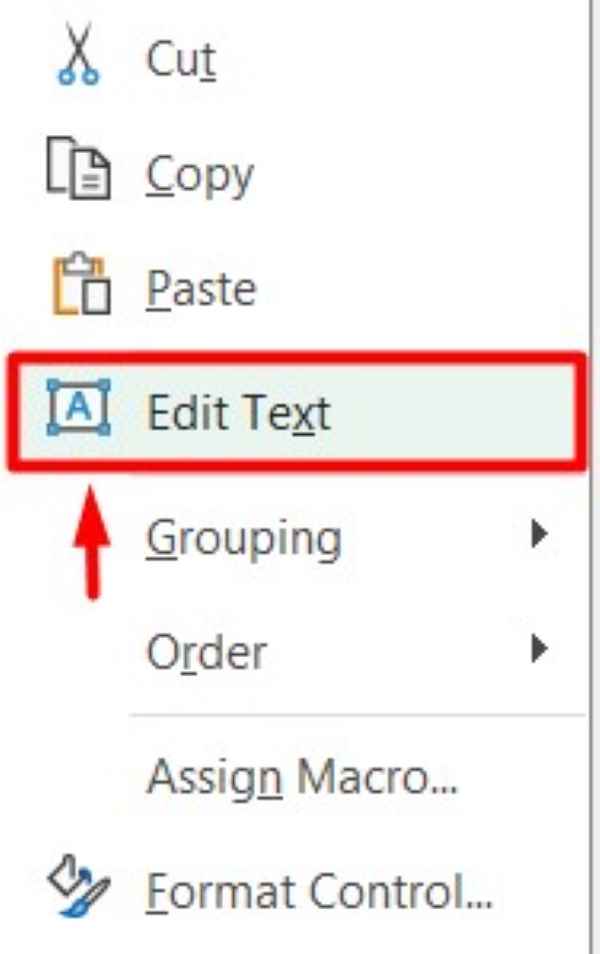
A context menu will appear; select “Edit Text” from this menu. The text in the checkbox will become editable. Type your desired label, then click outside the checkbox or press Enter to apply the change.
4. Duplicate the Checkbox if Needed
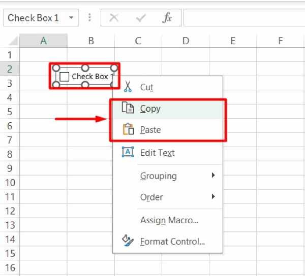
If you need multiple checkboxes, you can easily duplicate the existing one. Click on the checkbox to select it. Press “Ctrl+C” to copy the checkbox, then press “Ctrl+V” to paste it. A new checkbox will appear, which you can drag to your desired location. Repeat this process to create as many checkboxes as you need.
5. Link the Checkbox to a Specific Cell
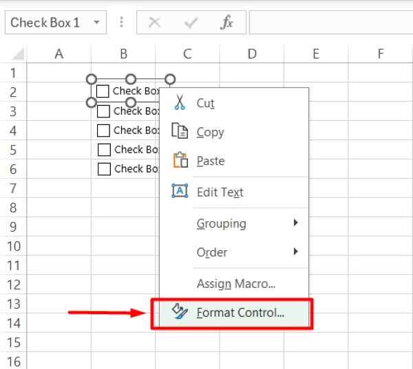
To make the checkbox functional, link it to a cell. Right-click on the checkbox and select “Format Control” from the context menu. In the “Format Control” dialog box, go to the “Control” tab.
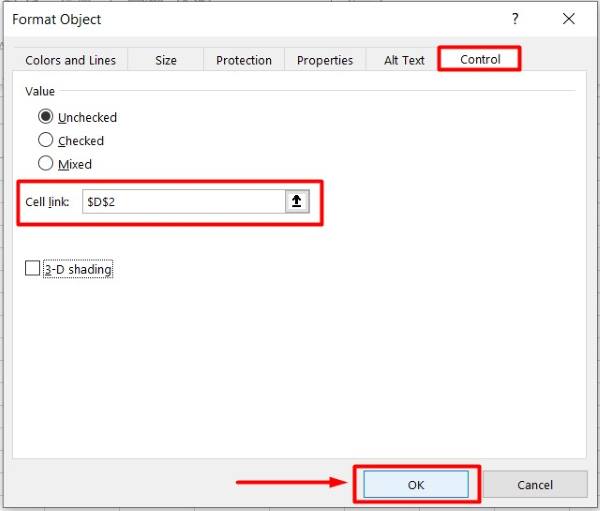
In the “Cell link” field, click the small icon to the right, then click on the cell in your worksheet that you want to link to the checkbox. Click “OK”.
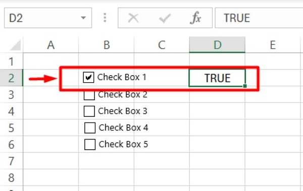
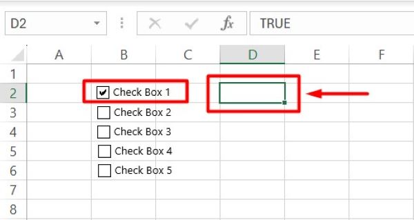
The linked cell will now display TRUE when the checkbox is checked and FALSE when it is unchecked.
6. Format the Linked Cells for Clarity
To improve the appearance of your worksheet, you can hide the TRUE/FALSE text in the linked cells. Select the cells that are linked to the checkboxes. Right-click on the selected cells and choose “Format Cells”.
In the “Format Cells” dialog box, go to the “Number” tab. Select “Custom” from the list on the left. In the “Type” field, enter three semicolons (“;;;“) and click “OK”.
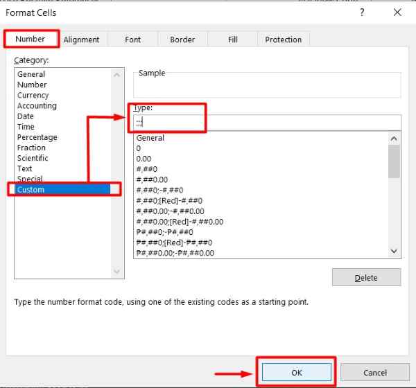
This will make the TRUE/FALSE text invisible in the linked cells. To ensure you don’t lose your work, save your workbook. Your workbook, complete with checkboxes, is now saved and ready for use.
We hope you now have a better understanding of how to put a checkbox in Excel. If you enjoyed this article, you might also like our article on how to insert gridlines in Excel or our article on ways to create list box in Excel.

