Compare Two Tables in Excel (Easiest Way in 2025)
In this article, we will explore how to compare tables in Excel. Simply follow the steps below.
How to Compare Two Tables in Excel
To compare tables in Excel, we will work with a dataset containing product categories in columns A and D, and their corresponding sales figures in columns B and E for Store A and Store B, respectively. Follow the steps below.
1. Select Store A’s Sales Data
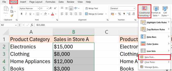
Start by selecting the cells from B2 to B6, which contain Store A’s sales figures. This selection will be the focus for applying the conditional formatting.

2. Access Conditional Formatting Options
Navigate to the ‘Home’ tab in Excel and click on ‘Conditional Formatting’. From the dropdown menu, select ‘New Rule’ to set up a new formatting condition.
3. Set Up the Comparison Formula
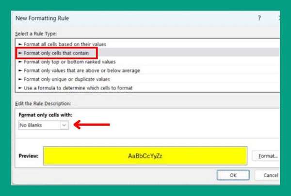
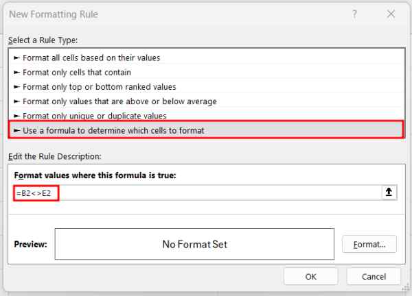
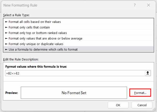
In the ‘New Formatting Rule‘ dialog, choose ‘Use a formula to determine which cells to format’. Enter the formula =B2<>E2 in the formula box. This formula checks if the sales figure in Store A (column B) does not match the corresponding figure in Store B (column E), indicating a discrepancy.
4. Choose a Highlighting Format
After inputting the formula, click on the ‘Format’ button within the ‘New Formatting Rule’ dialog.
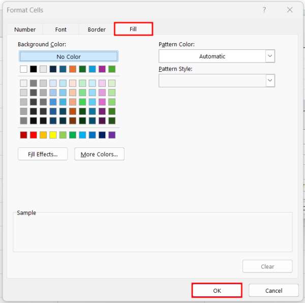
In the format settings, select the ‘Fill’ tab and choose a bright color, like yellow. This visual cue marks differences in sales figures clearly. Click ‘OK’ to apply your formatting choice.
5. Select Store B’s Data for Comparison
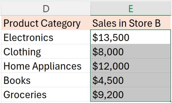
Apply similar steps to store B. Select the range E2 to E6 in Store B to apply the conditional formatting.
6. Apply Conditional Formatting with a Specific Formula in Store B
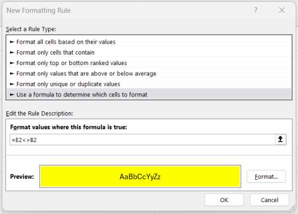
Use the conditional formatting rule with the formula `=E2<>B2`, which compares Store B’s data against Store A’s. This keeps your comparison consistent and visually marks all differences in both columns.
To maintain consistency with Store A, choose a yellow highlight for these differences.
7. Examine Highlighted Differences to Spot Sales Discrepancies
After applying conditional formatting, examine the highlighted cells in both Store A and Store B’s tables. Reviewing these highlights allows you to quickly spot where sales figures differ between the stores.

We hope that you now have a better understanding of how to compare two tables in Excel. If you enjoyed this article, you might also like our article on how to compare two columns in Excel using VLOOKUP or our article on how to compare strings in Excel.

