How to Freeze Second Row in Excel (Easiest Way in 2024)

In this article, we will show you how to freeze the second row in Excel. Simply follow the steps below.

Freeze Second Row in Excel

Follow the steps below on how to freeze the second row in Excel.

1. Select the Third Row to Prepare for Freezing

Click on the number of the third row on the left side of the Excel window to select it. This selection highlights the entire row. By selecting the third row, you instruct Excel to freeze everything above it, which includes both the first and second rows.

2. Go to the View Tab in the Ribbon

At the top of your Excel window, find and click on the “View” tab. This tab is part of the ribbon and contains several options related to how you view and interact with your worksheet. Clicking on this tab will display different viewing options.

3. Find and Click the Freeze Panes Option

Within the View tab, locate the “Freeze Panes” button. It is typically found in the “Window” group of options. Click on this button to reveal a dropdown menu with different options for freezing rows and columns.

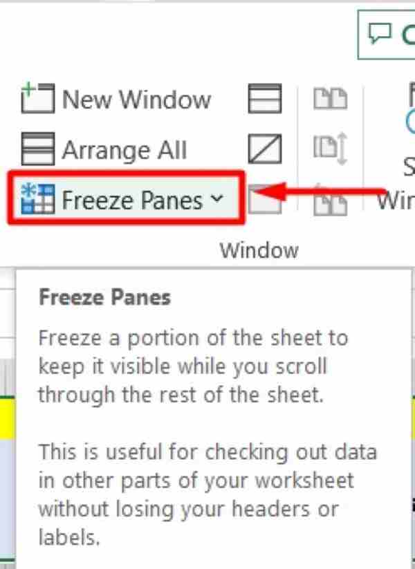
4. Select Freeze Panes from the Dropdown Menu

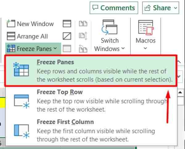
From the dropdown menu that appears when you click on “Freeze Panes,” select the “Freeze Panes” option at the top of the list. This action will freeze the rows above your selected row, specifically the first and second rows.

5. Verify the Second Row is Frozen

To verify that the second row is frozen, scroll down your Excel sheet. You should see that both the first and second rows remain visible at the top of the window even as you scroll further down the page.

We hope you now have a better understanding of how to freeze the second row in Excel. If you enjoyed this article, you might also like our article on how to freeze second column in Excel or our article on how to split a number in Excel.