How to Cross Reference Two Lists in Excel (2025 Guide)
In this article, we will show you how to cross reference two lists in Excel. Read on to learn more!
Cross Reference Lists in Excel
Cross-referencing lists in Excel is useful for comparing and analyzing data to maintain accuracy and consistency in your datasets. We will explore various methods such as Conditional Formatting, MATCH Function, VLOOKUP Function, COUNTIF Function, Power Query, and Array Formulas to efficiently cross-reference two lists in Excel.
Method 1: Using Conditional Formatting
To cross reference two lists in Excel using conditional formatting, follow these steps:
1. Prepare Your Lists
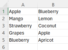
Ensure that your lists are in two separate columns. For example, List 1 in Column A and List 2 in Column B.
Here’s a sample dataset of fruits:
2. Select List 1
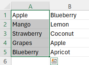
Click the first cell in List 1, drag down to select all the cells in that list.
3. Open Conditional Formatting
Go to the Home tab. Click on Conditional Formatting. Select New Rule.
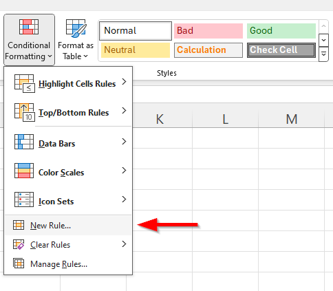
4. Set Up the Rule
Choose “Use a formula to determine which cells to format”.
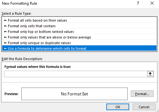
Enter the formula:
=COUNTIF(B:B, A1)>0

This formula checks if the value in List 1 (A1) appears in List B. Click ‘Format”, choose a fill color for highlighting, and press “OK”.
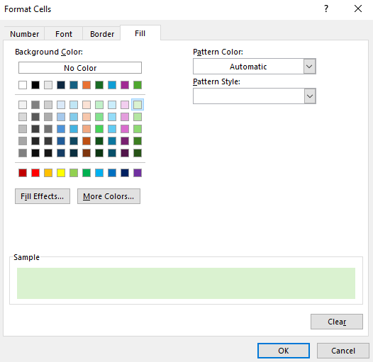
4. Apply and Check
Click “OK” again to apply the rule. Matching items in List 1 will now be highlighted.
Here’s what our example looks like:
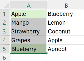
Method 2: Using the MATCH Function
The MATCH function searches for a specified item in a range and returns the relative position of that item. To cross reference two lists using this function, follow these steps:
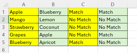
1. Enter the MATCH Formula
In Column C, next to the first cell of Column A, enter the following formula to find matches from Column A in Column B:
=IF(ISNUMBER(MATCH(A1, B:B, 0)), “Match”, “No Match”)
Drag the fill handle down to copy this formula for all cells next to list A.
2. Apply the Formula for the Second List
In Column D, next to the first cell of Column B, use this formula to find matches from Column B in Column A:
=IF(ISNUMBER(MATCH(B1, A:A, 0)), “Match”, “No Match”)
Drag the fill handle down to copy the formula for all corresponding cells next to list B.
Method 3: Using VLOOKUP
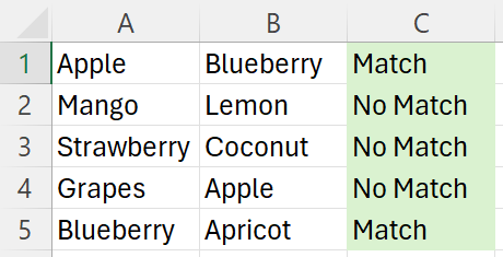
VLOOKUP can be used to find specific data in one column and bring it into the current column based on a match. In Column C next to the first cell of Column A, enter:
=IF(ISERROR(VLOOKUP(A1, B:B, 1, FALSE)), “No Match”, “Match”)
Copy the formula down to match the length of your list. The formula virtually works the same as the MATCH function.
Method 4: Using COUNTIF Function
This function helps identify if an item in one list appears in the other list by counting occurrences.
1. Prepare Your Lists
List 1 in Column A and List 2 in Column B.
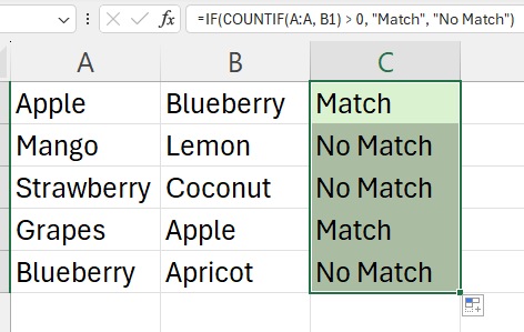
2. Enter the COUNTIF Formula
In Column C next to the first cell of Column A, enter:
=IF(COUNTIF(B:B, A1) > 0, “Match”, “No Match”)
Drag down the fill handle to copy the formula for all cells in List 1.
Method 5: Using Power Query
Power Query is a useful tool in Excel for merging and comparing lists with advanced queries.
1. Load Your Data into Power Query
Select each list, go to the “Data” tab, and choose “From Table/Range” to load each list into Power Query.

2. Merge Queries
With the data loaded in the Power Query Editor, click “Merge Queries” > “Merge Queries as New”.

3. Set Up Merge Settings
In the merge window, choose List 1 as the primary table and List 2 as the secondary table. For the merge type, select “Inner Join” to find names that appear in both lists.
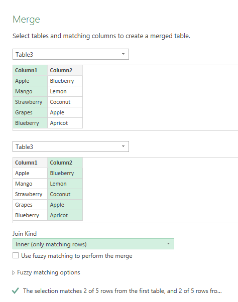
Once you configure your merge settings, click “OK”. The merged table should show the fruits found in both lists.

4. Apply and Close
Close and load the Power Query back into Excel.

Method 6: Using Array Formulas
Array formulas can provide powerful data processing capabilities for cross-referencing lists.
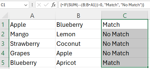
1. Setup Your Lists
For our example, we will input List 1 in Column A and List 2 in Column B.
2. Enter the Array Formula
In Column C next to List 1, enter the following formula and press Ctrl + Shift + Enter to create an array formula:
=IF(SUM(–(B:B=A1))>0, “Match”, “No Match”)
This formula must be entered as an array formula to work properly across multiple cells.
We hope that you now have a better understanding of how to cross reference two lists in Excel. If you enjoyed this article, you might also like our articles on how to remove a circular reference in Excel and how to find circular references in Excel.

