How to Show Number and Percentage in Excel Bar Chart in 2024

In this article, we will show you how to show the number and percentage in an Excel bar chart. Read on to learn more!

How to Show the Number and Percentage in an Excel Bar Chart

To show the number and percentage in an Excel bar chart, follow the steps below:

1. Input Your Data

Here is a sample dataset of sales figures for different products, organized in a table.

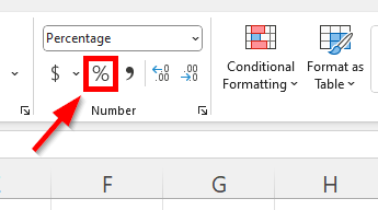
Make sure to convert the percentage column formulas to percentages in Excel by formatting the cells (click the percent sign in the Number section under the Home tab).

2. Insert a Bar Chart

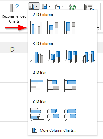
Select your data range excluding the percentage formula results. Go to the Insert tab, click on Bar Chart, and choose your preferred type of bar chart (e.g., Clustered Column).

3. Add Data Labels

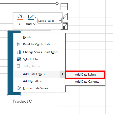
Click on the chart to select it. Right-click on the data bars and select Add Data Labels.

Right-click on the newly added labels, choose Format Data Labels.

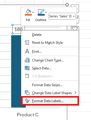
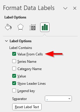
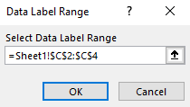
In the Format Data Labels pane, choose Value From Cells and select the range that contains the percentages. In our example, it would be =Sheet1!$C$2:$C$4. Make sure the Value is checked under the Label Options to display both details on your chart.

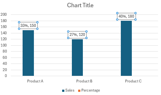
Here’s what our bar chart looks like with numbers and percentages:

We hope that you now have a better understanding of how to show the number and percentage in an Excel bar chart. If you enjoyed this article, you might also like our articles on how to make a bar chart in Excel with percentages and how to add a line to a bar chart in Excel.