Compare Two Columns in Excel and Highlight Matches (2025)
In this article, we will show you how to compare two columns in Excel and highlight matches. Simply follow the steps below.
How to Compare Two Columns in Excel and Highlight Matches
Follow the steps below on how to compare two columns in Excel and highlight matches.
1. Load Your Data into Two Columns
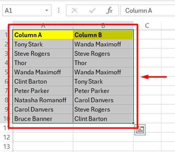
Load your data into two columns in Excel. For example, if you have a list of names, put one set of names in Column A and another set in Column B. Ensure both columns are aligned properly and have the same format.
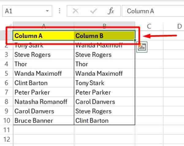
2. Select the Range of Cells to Compare
Select the range of cells in Column A that you want to compare with Column B. For instance, click and drag to highlight cells A1 to A10 or B1 to B10 if your data is in these cells. Make sure to select all the cells you want to compare.
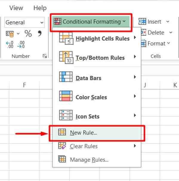
3. Navigate to Conditional Formatting Options
Go to the “Home” tab on the Excel ribbon at the top. Find the “Conditional Formatting” button in the Styles group. Click on it to open the dropdown menu. From the dropdown, select “New Rule” to create a new formatting rule.
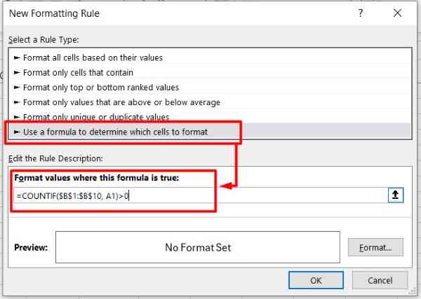
4. Enter Formula to Highlight Matching Cells
In the “New Formatting Rule” dialog box, select “Use a formula to determine which cells to format.” In the formula box, enter `=COUNTIF($B$1:$B$10, A1) > 0`. This formula checks if each cell in Column A is found in the range B1 to B10. Adjust the ranges if your data is in different cells.
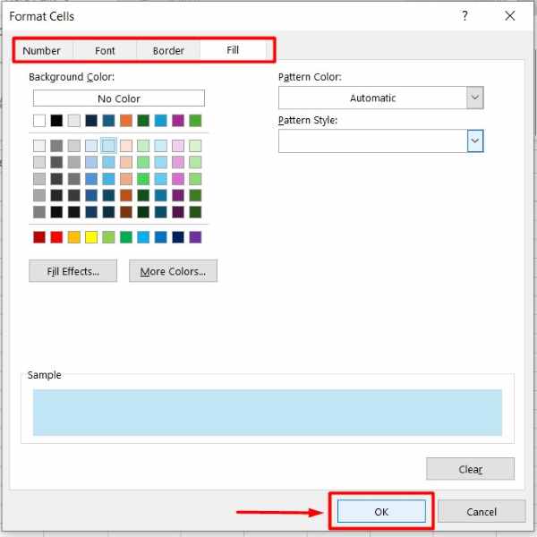
5. Choose Highlighting Format for Matches
Click the “Format” button to open the Format Cells dialog box. Here, you can choose how you want to highlight the matching cells. You can select a fill color, change the font color, or apply a border. Pick a format that will make the matches easy to see, then click “OK.”
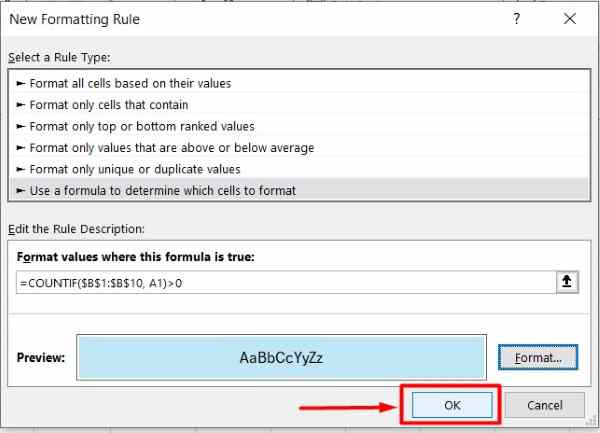
6. Confirm and Apply the Conditional Formatting Rule
Click “OK” in the “New Formatting Rule” dialog box to apply the rule. Excel will now highlight the cells in Column A that have matching values in Column B based on the formatting you selected.
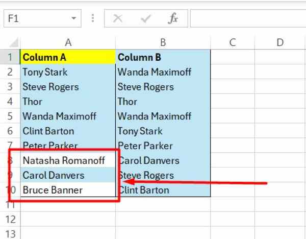
7. Verify Highlighted Matches in Column A
Look at the cells in Column A to ensure they are highlighted correctly. The highlighted cells should match the values in Column B. If some matches are missing or incorrect, double-check the formula and ranges used. Adjust as needed to ensure accuracy.
We hope you now have a better understanding of how to compare two columns in excel and highlight matches. If you enjoyed this article, you might also like our article on ways to how to highlight selected row in Excel or our articles on how to highlight highest value in Excel.