How to Count Number of Duplicates in Excel (Easiest Way in 2025)
In this article, we will explore how to count the number of duplicates in Excel. Simply follow the steps below.
Count the Number of Duplicates in Excel
To count the number of duplicates in Excel, you can use two of the most common methods: the ‘Filter Option’ technique and the ‘COUNTIF’ Function. We will discuss how to use each method in the following sections.
Method 1: Using the Filter Option to Find Duplicates
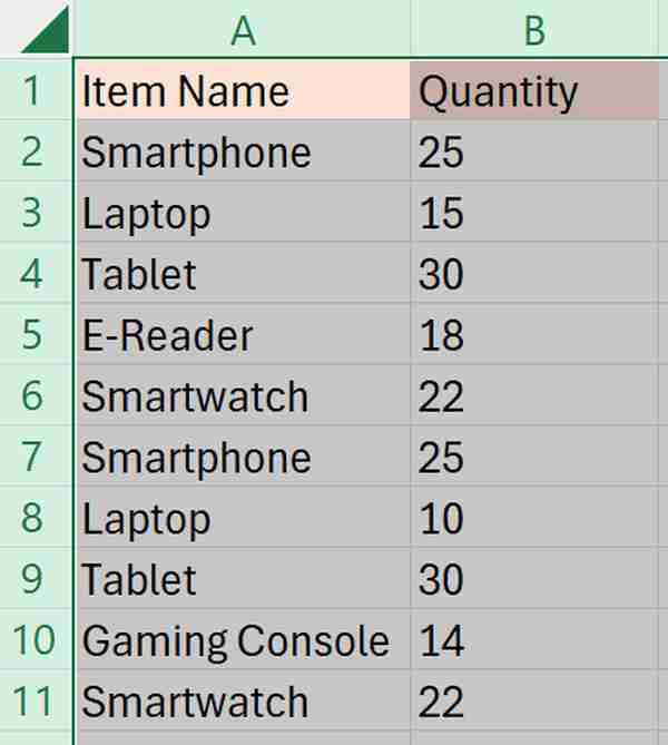
To count the number of duplicates in Excel, we will work with a dataset containing various electronic items. Follow the steps below:
1. Highlight the Entire Column to Check for Duplicates
Click on the letter at the top of the column that includes the data you want to inspect. This action highlights the entire column. For instance, if you’re checking ‘Item Name’ for duplicates, click on the column labeled ‘A’ at the top.
2. Turn on Filtering to Manipulate Data View
Navigate to the ‘Data’ tab located in the Excel ribbon at the top of the screen and select ‘Filter.’ This action adds small dropdown arrows in the headers of each column, enabling you to sort or filter the data based on content.

3. Sort Data Alphabetically to Group Similar Items
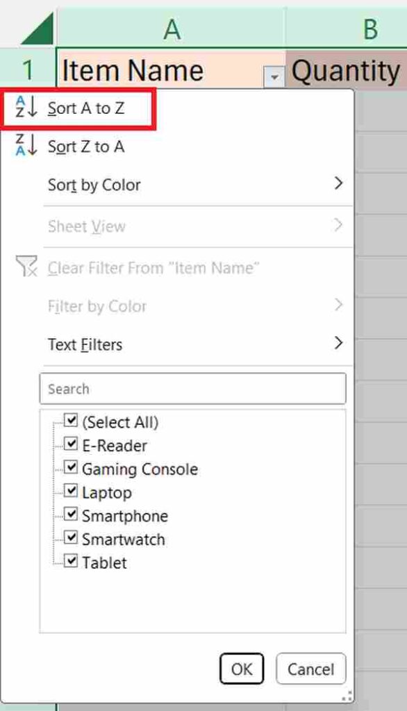
Click the dropdown arrow that appears in the header of your selected column after enabling filters. Select “Sort A to Z” from the dropdown menu. Sorting the data alphabetically groups identical or similar items together.
4. Manually Scan and Identify Duplicates in the Sorted List
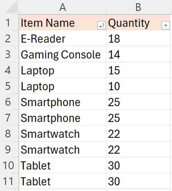
After sorting, scroll through your column to examine the data for duplicate entries. Look specifically for consecutive rows where the item names are identical as these are your duplicates.
Method 2: Using the COUNTIF Function to Quantify Duplicates
Here’s how to count the number of duplicates in Excel using the COUNTIF function.
1. Insert COUNTIF Formula to Count Occurrences
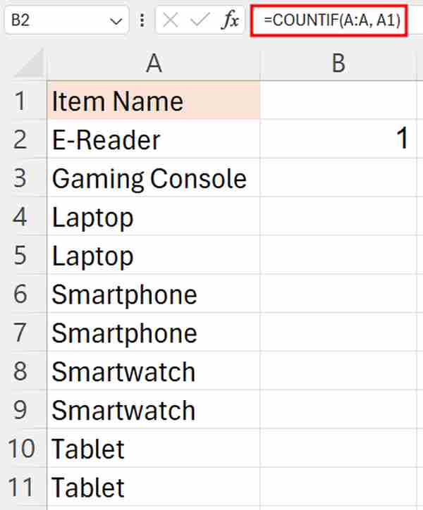
In our example, we have a list of electronic items from cells A2 to A11. You want to identify duplicate entries based on the item name.
In the column immediately to the right of your data (In our case, it’s cell B2), enter the formula =COUNTIF(A:A, A1). This formula counts how many times the value in the first cell (A1) appears throughout column A.
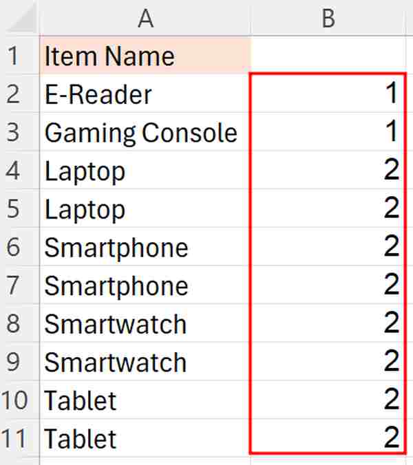
2. Copy the COUNTIF Formula Down the Column
Click on the small square at the bottom right corner of the cell where you just entered the formula. Drag it down through the column to apply the formula to other cells. This action replicates the formula for each row.
3. Apply a Filter to the COUNTIF Column
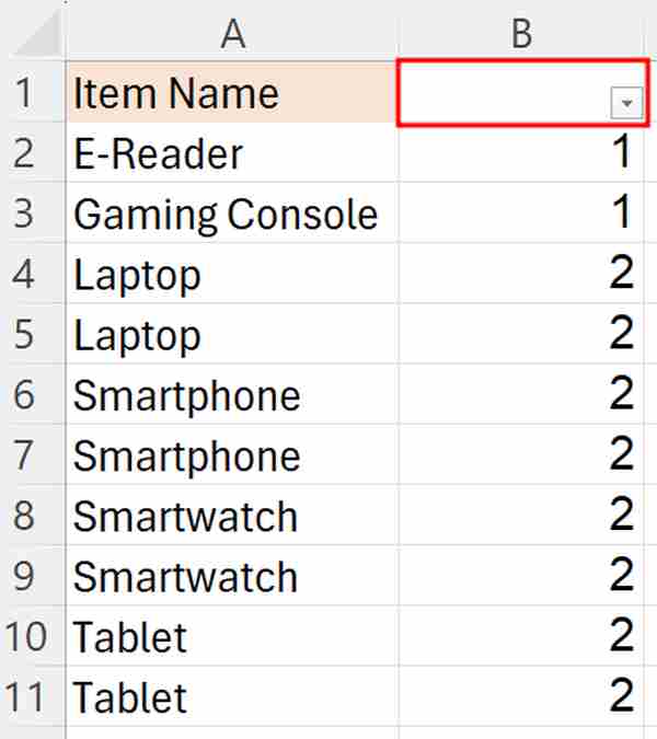
Once the formula is applied down column B, you’ll need to filter the results to identify duplicates. Navigate to the ‘Data’ tab located in the Excel ribbon at the top of the screen and select ‘Filter.’

Go to the column header of column B and click the dropdown arrow. This will open the filter options for that column.
4. Set Filter to Show Only Duplicates
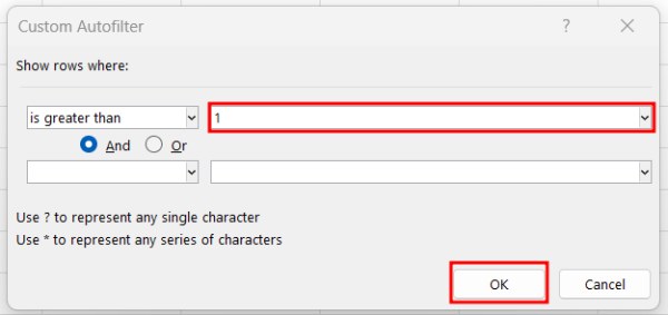
In the filter menu, choose ‘Number Filters’ and then select ‘is Greater Than’. In the box that appears, enter ‘1’. This setting will filter the column to show only the cells where the count is greater than 1, which indicates duplicate entries. Click ‘OK’ to apply this filter setting.
5. See Duplicate Results
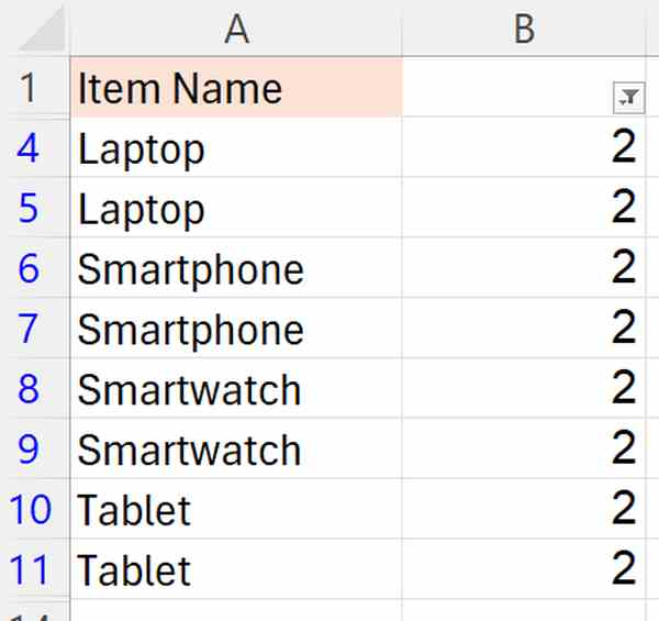
Now, your Excel sheet will display only rows where the item name appears more than once.
We hope that you now have a better understanding of how to count the number of duplicates in Excel. If you enjoyed this article, you might also like our article on how to generate random numbers in Excel without duplicates within a range or our article on how to hide duplicates in Excel.

