How to Filter by Date in Excel (Easiest Way in 2025)
In this article, we will explore how to filter by date in Excel. Simply follow the steps below.
How to Filter Dates in Excel
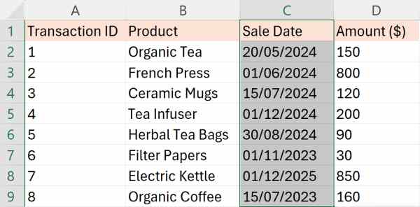
To filter by dates in Excel, we will work with a dataset containing sales transactions that include some errors with future dates. This dataset includes transaction IDs in Column A, product names in Column B, sale dates in Column C, and amounts in Column D. Follow the steps below:
1. Select the Column Containing Dates
Locate and click on the column header that reads “Sale Date,” indicating where the dates are stored. This action highlights the entire column.
2. Activate Filtering for Your Data
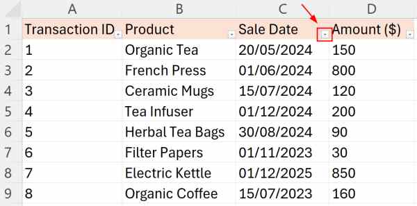
From the Excel ribbon at the top of your screen, go to the “Data” tab and find the “Filter” button. Click on it to activate dropdown arrows on each column header. This will enable the filtering feature for each column.

3. Access the Date Filter Options
Click on the dropdown arrow that now appears in the “Sale Date” column header.
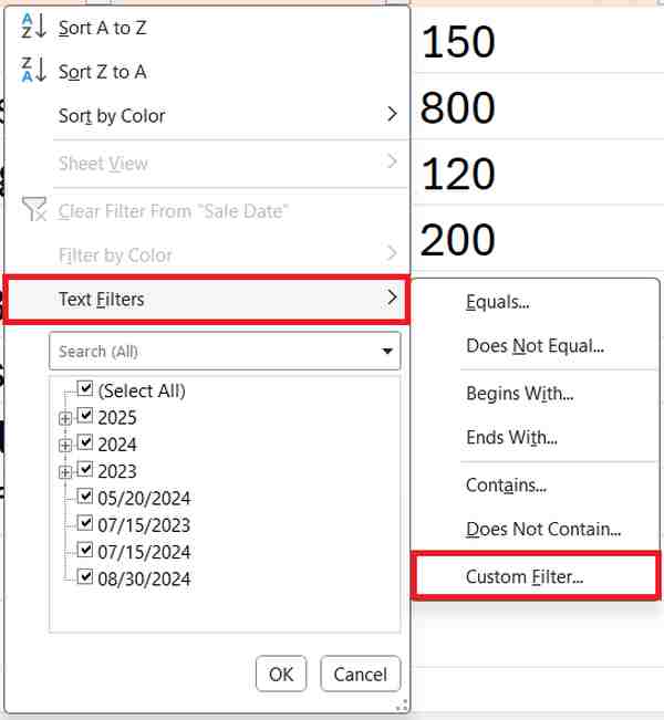
Look for the submenu labeled “Text Filters” and choose “Custom Filter”. This will open a dialog where you can specify more detailed criteria for filtering dates.
4. Specify the Date Range for Filtering
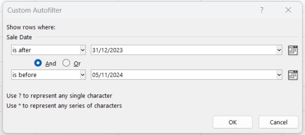
In the Custom AutoFilter dialog, select “is after” in the first dropdown menu and enter the start date for the filter. In our case, let’s choose December 31, 2023 (31/12/2023) as the start date.
Click “And” to add a second condition. Select “is before” in the second dropdown menu and enter the end date. Let’s choose November 5, 2024 (05/11/2024). Click “OK” to apply the filter.
5. Review Sale Date Results
It will now filter out any transactions that fall outside your specified date range of December 31, 2023, to November 5, 2024, such as future dates incorrectly entered.

We hope that you now have a better understanding of how to filter by date in Excel. If you enjoyed this article, you might also like our article on how to add a drop-down filter in Excel or our article on how to filter by color in Excel.

