Delete Filtered Rows in Excel (Easiest Way in 2025)
In this article, we will show you how to easily delete filtered rows in Excel. Simply follow the steps below.
How to Delete Filtered Rows in Excel Using Filter Option
Follow the process below to delete filtered rows in Excel using the filter option.
1. Apply a Filter to Your Data
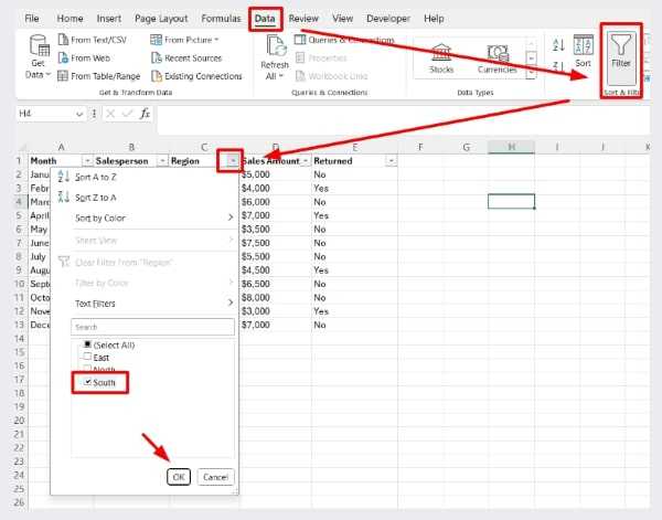
Open your Excel file and highlight the data range where you want to delete rows. Then, go to the “Data” tab and click on “Filter” to apply a filter to your data. Click on the drop down arrow of the column you want to filter. Unselect “Select All” and then choose the filter you want to show. Click the “OK” button to apply the filter.
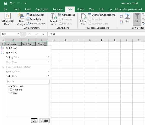
2. Select the Filtered Rows You Want to Delete
Click on the row number header on the left side of the spreadsheet to select the entire row. You can select multiple rows by holding down the “Ctrl” key while clicking on additional row numbers.
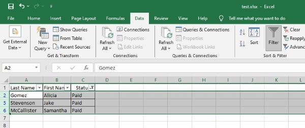
3. Delete the Filtered Rows
Once you’ve selected the filtered rows, right-click on any of the selected row numbers and choose “Delete Row” from the context menu. Excel will prompt you to confirm the deletion. Click “OK” to permanently delete the filtered rows from your spreadsheet.
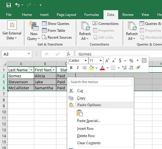
4. Clear the Filter (optional)
If you no longer need the filter applied to your data, you can clear it by clicking on the filter icon in the column header of the filtered column and selecting “Clear Filter from [Column Name]”. This will display all rows in your spreadsheet again.
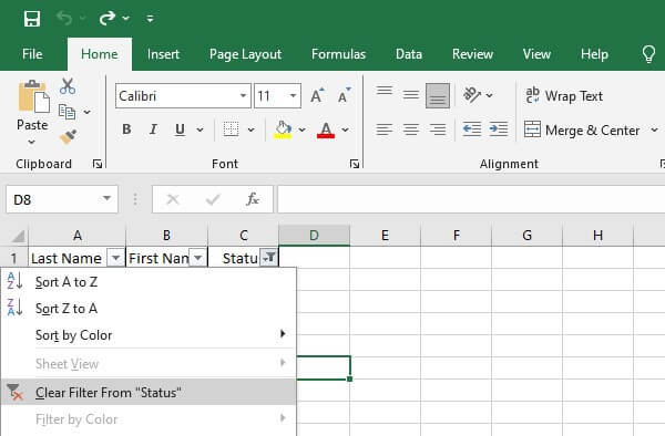
How to Filter and Delete Rows Using The ‘Go To Special’ Feature
Follow the process below to delete filtered rows in Excel using the ‘Go To Special’ feature.
1. Apply a Filter to Highlight Specific Data Rows
In our example, we will be using the “Monthly Sales Data” to apply a filter on the “Region” column to show only sales from the “South” region. Select Data > Filter. Click the filter arrow in the column “Region” and selecr
2. Access ‘Go To Special’ to Select Filtered Data
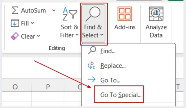
After filtering, select any cell within the filtered range. Then, go to “Home” -> “Find & Select” -> “Go To Special.”

3. Select Only Visible Cells Using ‘Go To Special’
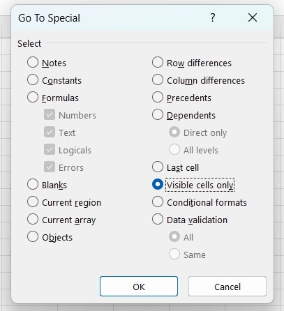
In the Go To Special dialog box, select “Visible cells only” and click “OK.” This action will highlight all cells that are not hidden by the filter.
4. Delete the Selected Visible Rows
With the cells still selected, press Ctrl + – (Control key and the minus key) to delete the rows. Confirm the deletion if prompted by Excel.

How to Delete Only Unfiltered Rows in Excel Using the ‘Advanced Filter’
Follow the steps below to delete only unfiltered rows in Excel using the Advanced filter.
1. Set Up Criteria Range Above Your Dataset
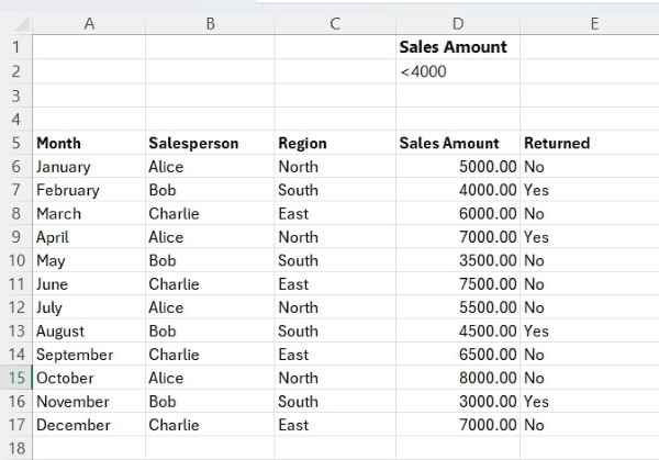
Start by creating a criteria range directly above your dataset to specify which rows to filter. For instance, if your dataset starts from row 1, set up the criteria range in row 1. This range should include the same column headers as in your dataset.
2. Apply Advanced Filter to Display Only Rows Matching Criteria
Go to the Data tab and click on Advanced in the “Sort & Filter” group.

In the Advanced Filter dialog box, choose “Filter the list, in-place.” For the ‘List range’, select the entire dataset including the headers. For the ‘Criteria range’, select your newly created criteria range, including the headers.
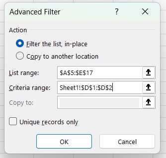
3. Select Rows Displayed by the Advanced Filter
After applying the filter, only rows where the “Sales Amount” is less than $4,000 will be visible. Select these rows by clicking on the header of the first column of your dataset and dragging down to the last row displayed by the filter.

4. Delete Visible Rows Matching the Criteria
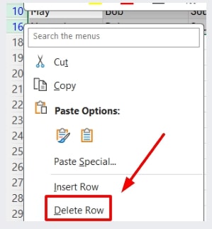
Right-click on one of the selected rows and choose “Delete Row” from the context menu. This action will delete all rows that are currently visible and match the filtering criteria, effectively removing sales records where amounts are less than $4,000.
We hope that you now have a better understanding on how to delete filtered rows in Excel.

