Add Drop Down List Filter in Excel (Easiest Way in 2024)

In this article, we will show you how to add drop down filters in Excel. Simply follow the steps below.

How to Add Drop Down Filters in Excel

To add drop down filters in Excel, simply follow the process below.

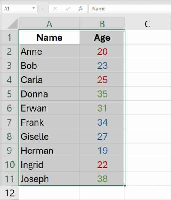
1. Select your data range.

Select the data range where you want to apply the filters. For example, if you have a list of names and corresponding ages, select both columns.

2. Go to the “Data” tab.

At the top of the Excel window, you’ll see different tabs like “Home,” “Insert,” “Page Layout,” etc. Click on the “Data” tab.

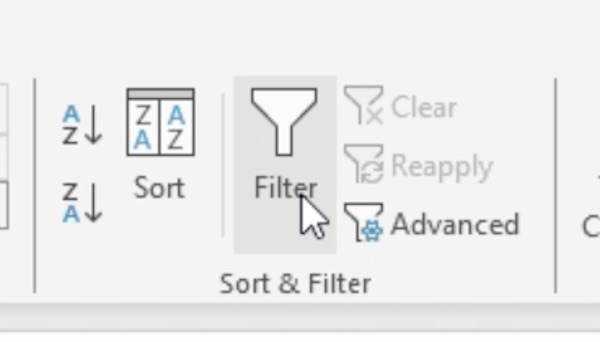
3. Click on “Filter” in the “Sort & Filter” group.

In the “Sort & Filter” group, you’ll find the “Filter” button. Click on it. This will add filter arrows to the top of each column in your selected data range.

4. Click on the filter arrow in the column header.

Move your mouse cursor to the top of the column where you want to add a drop-down filter. You’ll see a small filter arrow appear. Click on it.

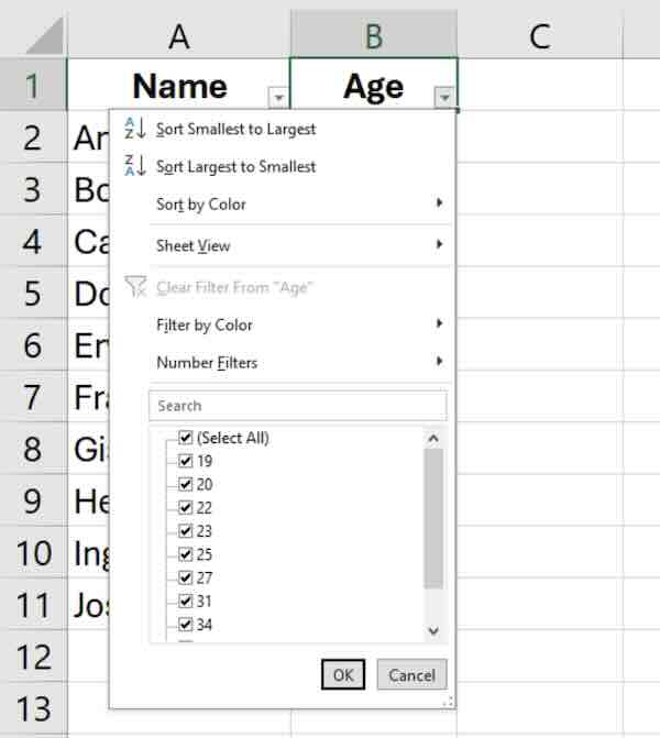
5. Select “Filter by Color” or “Filter by Cell Value.”

After clicking on the filter arrow, a dropdown menu will appear. Depending on what you want to filter, choose either “Filter by Color” or “Filter by Cell Value.”

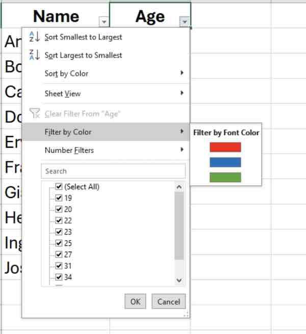
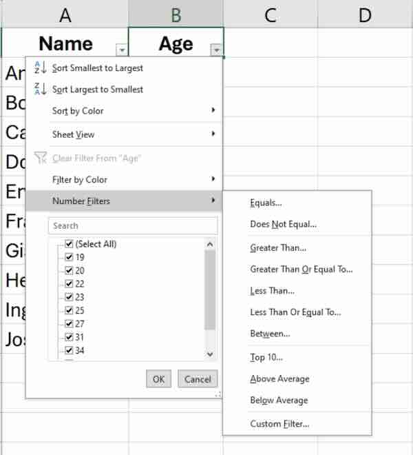
6. Choose your filtering criteria.

Once you’ve selected either “Filter by Color” or “Filter by Cell Value,” another menu will pop up. Here, you can specify your filtering criteria. For example, if you chose “Filter by Cell Value,” you can enter specific values you want to filter by.

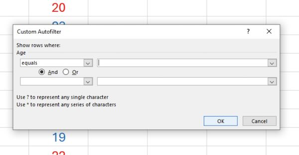
7. Click “OK” to apply the filter.

After specifying your filtering criteria, click the “OK” button. Excel will apply the filter, and you’ll see only the data that meets your criteria.

We hope you now have a better understanding of how to add a drop down list filter in Excel. If you enjoyed this article, you might also like our article on how to delete filter in Excel or our article on how to filter by date in Excel.