Fill Color Based on Value in Excel (Easiest Way in 2025)
In this article, we will learn how to fill color based on value in Excel by using conditional formatting. Simply follow the steps below.
Fill Color Based on Value in Excel Using Conditional Formatting
Follow the steps below to fill color based on value in Excel by using conditional formatting.
1. Select the Data Range
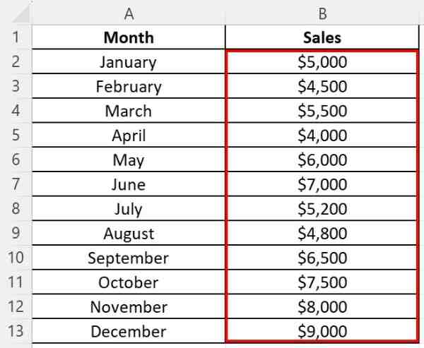
Let us consider a dataset of monthly sales figures for a store. For this example, we will select cell B2 then drag down to B13 to select all the sales data.
2. Apply Conditional Formatting
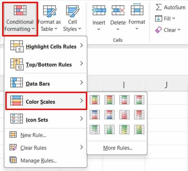
With the range B2 to B13 selected, go to the Home tab on the Ribbon. Click on Conditional Formatting from the Styles group. From the dropdown menu, select Color Scales to see different gradient styles. Choose a color gradient scale that suits your preference. For this example, we will choose Green Yellow Red Color Scale (green applies to the highest values, yellow to the middle values, and red to the lowest values).
3. Check the Applied Colors
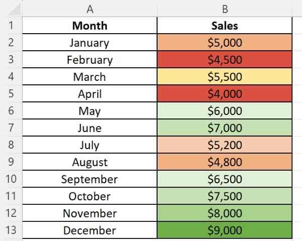
Look at your sales data and see the color gradient reflecting the value range. If the results aren’t what you expected, you can return to the Manage Rules dialog under conditional formatting and adjust the settings.
4. Customize the Formatting (Optional)
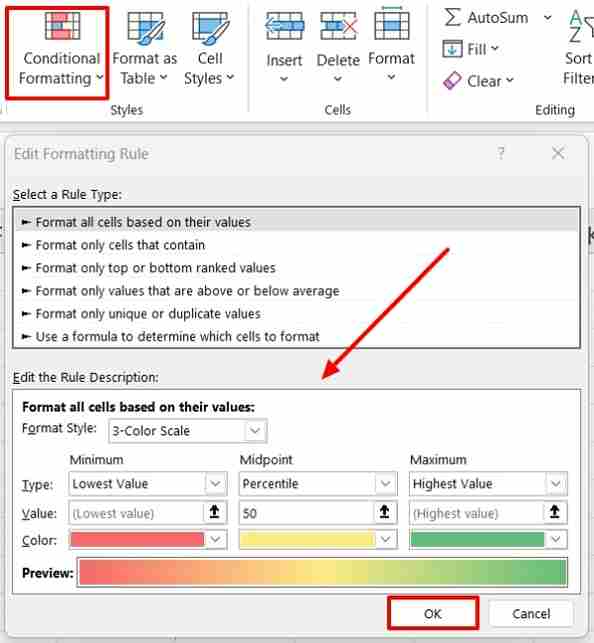
If you wish to customize the colors or the thresholds, go back to Conditional Formatting and select Manage Rules. In the Conditional Formatting Rules Manager, select the rule you’ve just created and click Edit Rule. You can adjust the minimum, midpoint, and maximum settings based on percent, number, formula, or percentile according to your data. You can also select the color for each point (minimum, midpoint, maximum) by clicking on the dropdown next to each and selecting a new color. Once done, click OK to close each window.
We hope that you now have a better understanding of how to fill color based on value in Excel. If you enjoyed this article, you might also like our article on how to use COUNTIF to count fill color in excel and our article on how to gradient fill across multiple cells in Excel .