How to Filter in Excel Based on a List (Easiest Way in 2025)
In this article, we will show you how to filter a list in Excel using the filter function and the advanced filter method. Simply follow the steps below.
Filter Excel Based on a List Using the Filter Function
Follow the steps below to filter Excel based on a list using the filter function.
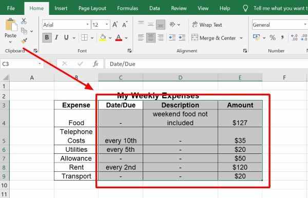
1. Highlight the Cells You Want to Filter
Highlight the cells containing the data you want to filter. For example, if you’re managing expenses, select the cells with dates, descriptions, amounts, and categories.
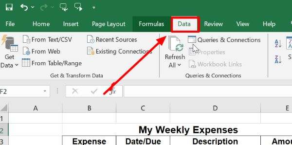
2. Access the “Data” tab
Click on the “Data” tab at the top of Excel. This tab has tools for organizing and analyzing your data, including filtering.
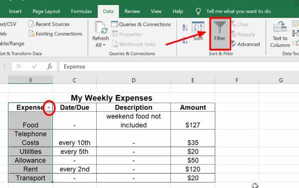
3. Click on “Filter”
In the “Data” tab, find “Sort & Filter” and click “Filter.” This adds filter arrows next to each column header in your selected data range.
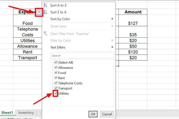
4. Specify filter criteria
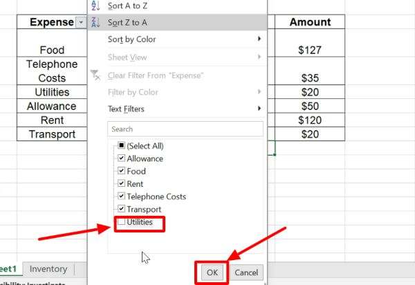
Click the filter arrow next to the column header you want to filter. Select filtering options from the dropdown menu. For instance, select a specific category like “Utilities” for expenses.
5. Activate the filter by clicking “OK”
Click “OK” or “Apply” to activate the filter. Excel hides rows that don’t meet the criteria. For instance, only expenses not categorized as “Utilities” will show.
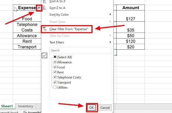
6. Optional: Clear the filter
To show all data again, click the filter arrow and select “Clear Filter.” This reverts to showing all expenses.
Filter Excel Based on a List Using the Advanced Filter
Follow the steps below to filter a list in Excel using the advanced filter method.
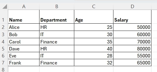
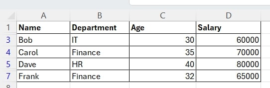
1. Open Your Excel File and Prepare Your Data
Open your Excel file. Ensure your data is in a table format with headers. This makes it easier to manage and filter.
2. Create a Criteria Range for Filtering
Decide which criteria you want to filter by. Copy the headers of the columns you want to filter. Paste these headers in an empty part of your worksheet. Under each header, list the specific criteria you want to filter.
Criteria Range: IT>30
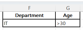
This criteria means you are looking for records in the IT department where the age is greater than 30.
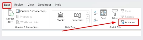
3. Access the Advanced Filter Option
Click on any cell within your data range. Go to the ‘Data’ tab on the Ribbon. Click ‘Advanced’ in the ‘Sort & Filter’ group.
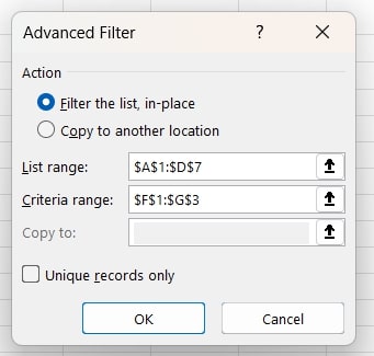
4. Configure the Advanced Filter Settings
In the ‘Advanced Filter’ dialog box, choose ‘Filter the list, in-place’ if you want to filter the data in the current location. Select ‘Copy to another location’ if you want to move the filtered data to a new location. In the ‘Criteria range’ field, enter the range where you listed your criteria.
Example:
List range: $A$1:$D$7
Criteria range: $F$1:$G$2
5. Apply the Advanced Filter
Click ‘OK’ in the ‘Advanced Filter’ dialog box. Your data will now be filtered based on the criteria you set. If you chose to copy the filtered data, it will appear in the location you specified.
6. Verify and Adjust the Filtered Data
Check the filtered data to ensure it meets your criteria. Make any necessary adjustments to your criteria range and reapply the filter if needed.
We hope that you now have a better understanding of how to filter in Excel based on a list. If you enjoyed this article, you might also like our article on how to filter unique values in Excel or our article on how to filter multiple columns in Excel.