Filter Horizontally in Excel (Easiest Way in 2025)
In this article, we will explore how to filter horizontally in Excel. Simply follow the steps below.
How to Filter Horizontally in Excel
Horizontal filtering in Excel can be achieved using two effective methods: the ‘FILTER Function’ and the ‘Transpose Option’. We will discuss how to use each method in the following sections.
Method 1: Using the FILTER Function
Follow the steps below to filter horizontally in Excel.
1. Use the FILTER Function to Display Products Priced Over $200 and In Stock
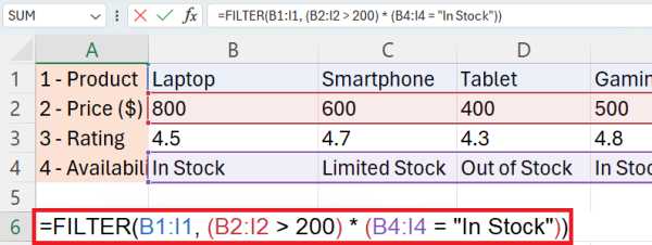
In our example, we have a dataset featuring a range of products arranged horizontally from cells B2 to I2, with corresponding prices, customer ratings, and availability statuses listed in the rows directly below. We want to filter this information horizontally, focusing specifically on products based on their price and availability.

Select a new cell where you want the filtered results to appear. In our case, we will use cell A6. Assuming prices are in row 2 and availability statuses are in row 4, type the FILTER function formula: =FILTER(B1:I1, (B2:I2 > 200) * (B4:I4 = “In Stock”)). This formula filters the row of product names based on the corresponding conditions set in the price and availability rows.
2. Execute the FILTER Function
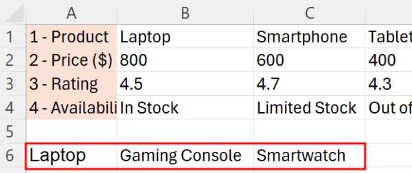
Press Enter after typing the formula. Excel will display horizontally the names of the products that are both priced over $200 and in stock, based on your criteria.
Method 2: Using the Transpose Option
To use horizontal filtering techniques in Excel, we will work with a dataset containing product names in Row 1 from cells B1 to I1, and corresponding details like prices, customer ratings, and availability statuses in Rows 2 to 4. Follow the steps below:
1. Transpose the Data to Vertical Format
First, select the entire dataset from A1 to I4. Copy the selected area, then right-click in a new location on your sheet (cell A6).
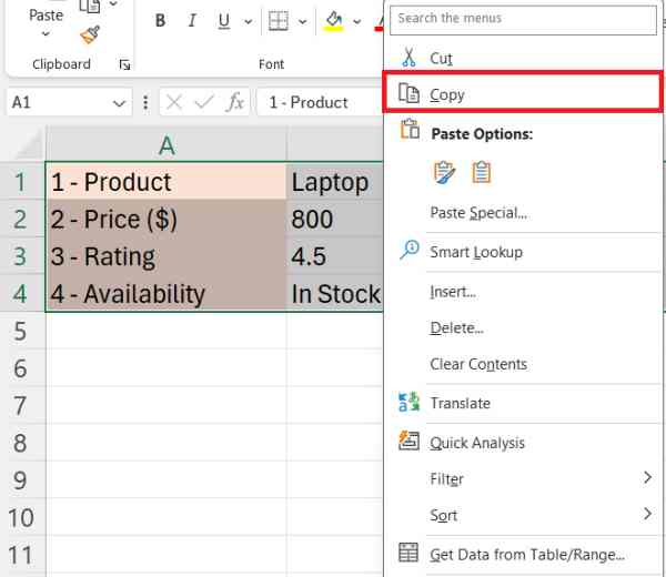
Go to ‘Paste Special’, and choose ‘Transpose’.
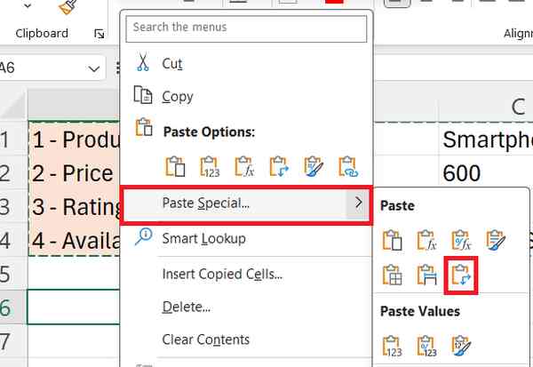
This will convert your horizontal data into a vertical column format, making it easier to apply vertical filters if needed.
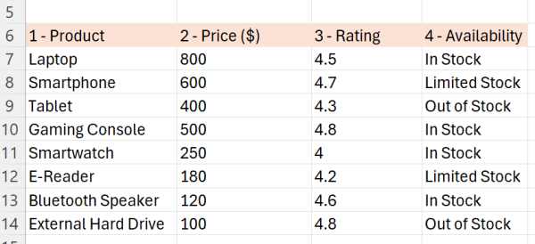
2. Apply Filters Directly to the Vertical Data
With your data now vertical, apply a standard filter. Highlight the column where the data is now placed, go to the ‘Data’ tab, and click on ‘Filter’. This enables filtering options at the top of the column.

In the dropdown menu, choose ‘Number Filters’ and then select ‘Greater Than’.
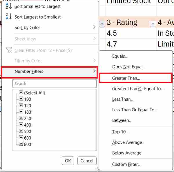
Enter ‘200’ in the field provided to set the condition for prices greater than $200.
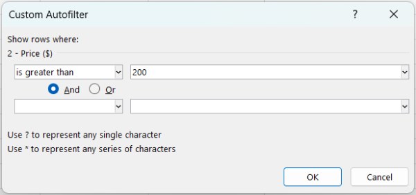
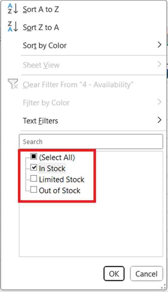
Next, apply a filter to the availability column. Click the dropdown arrow in the column header for availability. Uncheck ‘Select All’ to clear all selections, and then check ‘In Stock’ to filter for products that are currently available.
3. Review Filtered Vertical Data
Once the criteria are set, the spreadsheet will automatically update to display only the rows that meet both conditions: prices over $200 and availability marked as ‘In Stock’.

4. Copy and Transpose the Filtered Data Back Horizontally
Once your data is filtered, copy the filtered column by right-clicking and selecting ‘Copy’ or pressing Ctrl+C. Then, navigate to the location where you want to paste this data horizontally, such as cell A17. Right-click on cell A17, select ‘Paste Special’, and then choose ‘Transpose’. This action will paste the previously vertical data back into a horizontal layout.

We hope that you now have a better understanding of how to filter horizontally in Excel. If you enjoyed this article, you might also like our article on how to add filters to multiple columns in Excel or our article on how to filter and delete cells in Excel.

