How to Filter Strikethrough in Excel (Easiest Way in 2025)
In this article, we will show you how to filter strikethroughs in Excel. Simply follow the process below.
Filter Strikethrough in Excel
Filtering strikethroughs directly in Excel using built-in filtering options is not possible since Excel does not provide a direct filter for cell formatting like strikethrough. However, you can use a workaround by creating a helper column with a formula that identifies cells with strikethrough formatting. Follow the steps below.
1. Open Your Excel Spreadsheet with the Data Set
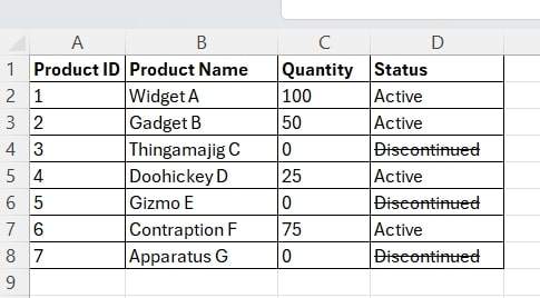
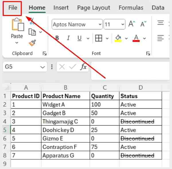
Open your Excel spreadsheet containing the data set you want to work with. Ensure the data is correct and ready for manipulation.
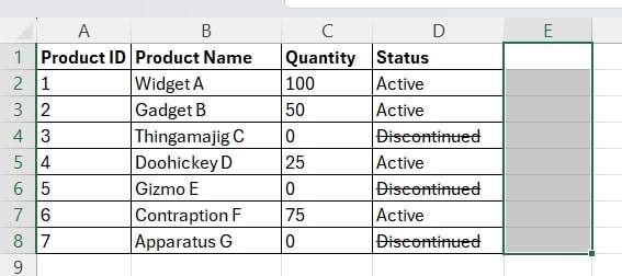
2. Add a Helper Column Next to Your Data
Insert a new column next to your data. This column will be used to identify cells with strikethrough formatting.
3. Open the VBA Editor
Enable the Developer Tab (if not already enabled):
Click on the “File” menu.
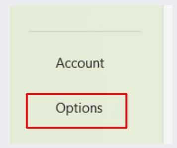
Select “Options.”
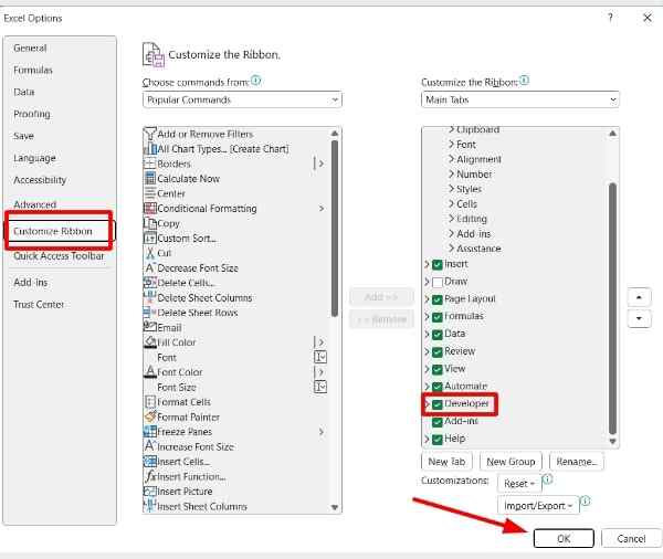
In the Excel Options dialog box, select “Customize Ribbon.” Check the box next to “Developer” in the right pane. Click “OK” to enable the Developer tab.
Open the VBA Editor:
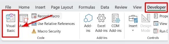
Go to the “Developer” tab in the Excel ribbon. Click on the “Visual Basic” button on the left side of the ribbon. This will open the VBA editor.
4. Insert a New Module
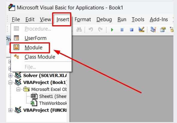
In the VBA editor, insert a new module by clicking Insert > Module. This is where you will write your custom function.
5. Write the VBA Function to Detect Strikethrough
Copy and paste the following VBA code into the module:
Function IsStrikethrough(cell As Range) As Boolean
Application.Volatile
IsStrikethrough = cell.Font.Strikethrough
End Function
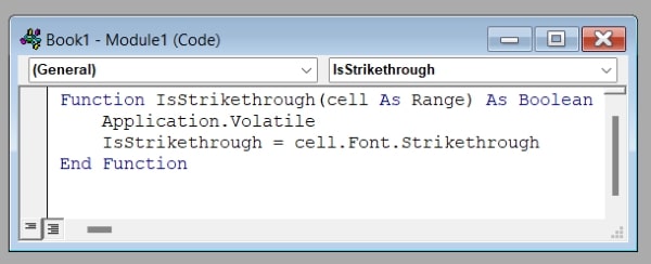
This function returns TRUE if the cell has strikethrough formatting and FALSE otherwise.
6. Use the Custom Function in Your Helper Column
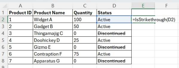
Close the VBA editor and return to your Excel spreadsheet. In the first cell of the helper column, use the custom function to check for strikethrough formatting. For example, if your data starts in cell D2, enter the following formula in the helper column (e.g., E2):
=IsStrikethrough(D2)
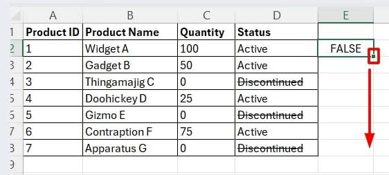
Drag the fill handle down to apply this formula to the entire column.
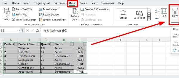
7. Enable Filtering on Your Data
Select the entire data set, including the headers and the helper column. Go to the “Data” tab in the Excel ribbon. Click on the “Filter” button in the “Sort & Filter” group. This will add drop-down arrows to each header cell, including your helper column.
8. Filter the Helper Column for Strikethrough
Click on the drop-down arrow in the header of the helper column. Filter the column to show only cells where the value is TRUE.
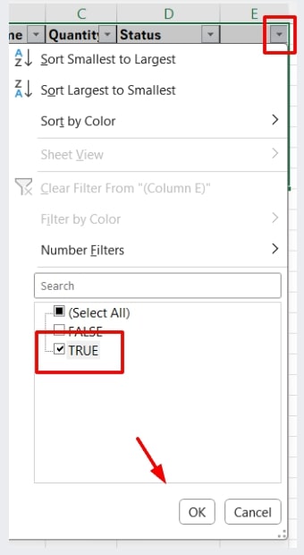
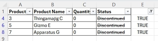
This will display only the rows where cells have strikethrough formatting.
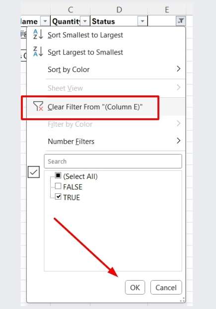
9. Clear the Filter to Show All Data Again
To show all data again, click on the filter arrow in the filtered column. Then, select “Clear Filter.”
We hope that you now have a better understanding of how to filter by strikethrough in excel. If you enjoyed this article, you might also like our article on how to filter wildcards in Excel and how to use our savings goal calculator in Excel.