How to Freeze Header in Excel (Easiest Way in 2024)

In this article, we will show you how to freeze headers in Excel. Simply follow the steps below.

How to Freeze Heading Row in Excel

Follow the steps below on how to freeze the heading ROW in Excel.

1. Identify the Heading Row

Locate the row in your worksheet containing the headings or labels for your data. This row typically includes titles for each column, such as “Name,” “Date of birth,” etc.

2. Select the Cell Below the Header Row

Choose the cell directly below the header row in your worksheet. Then, select the row right below the last row you want to freeze. For example, to freeze the Header Row, select cell A3 or the entire row 3.

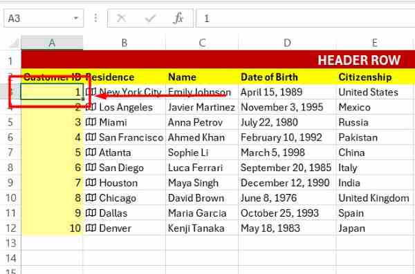
3. Access the “View” Tab in the Ribbon Menu

At the top of the Excel window, locate and click on the “View” tab in the ribbon menu. This tab contains options related to the appearance and layout of your spreadsheet. From the dropdown menu, select the “Freeze Panes” option. This will freeze the selected row (the heading row) at its current position in the Excel window, allowing it to remain visible as you scroll through your data.

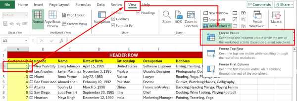
4. Confirm the Freeze Header in Excel

Scroll through your worksheet to ensure that the heading row remains fixed at its position in the window. You should be able to scroll through your data while still seeing the headings.

How to Freeze Column Headings in Excel

Follow the steps below on how to freeze COLUMN headings in Excel.

1. Locate the Column Headings

Find the row at the top of your spreadsheet with the column labels. These labels typically describe the content of each column, such as “ID,” Date,” “Product,” or “Price.” Click on the letter of the column directly to the right of the one with row labels.

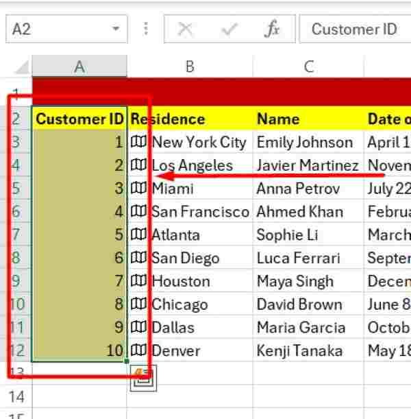
2. Navigate the “View” Tab” to Access Various Options

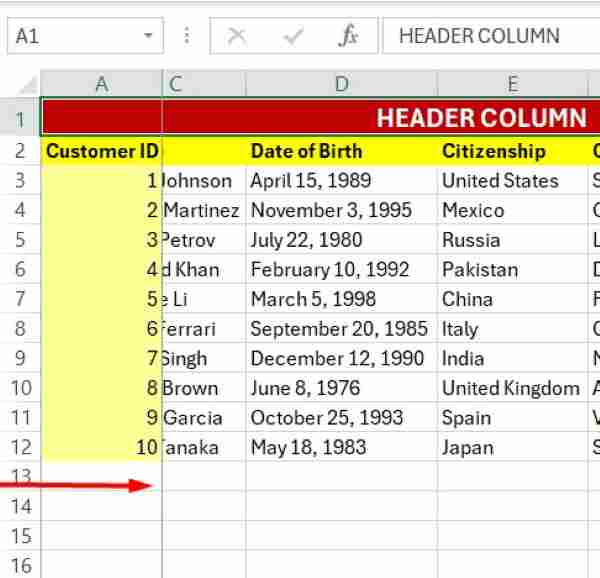
Go to the top of Excel and click on the “View” tab. Look for the “Freeze Panes” option. From the dropdown menu, select “Freeze First Column.” This option will lock the first column (containing the row labels) in place while you scroll horizontally.

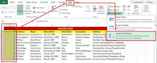
3. Check the Freeze Column Headings

Scroll horizontally to ensure the column headings stay visible as you navigate through your data. This confirms that the freezing process was successful.

We hope you now better understand how to freeze headers in Excel. If you enjoyed this article, you might also like our article on how to freeze titles in Excel or our article on how to freeze selected rows in Excel.