How to Save a Filter in Excel (Easiest Way in 2025)
In this article, we’ll explore how to save a filter in Excel to ensure efficient data management and easy access to customized views. Simply follow these steps outlined below.
How to Save a Filtered View in Excel
Here’s how to save filters in Excel and keep your filtering criteria when working with data. You’ll need to utilize the Custom View feature for this task. This powerful tool allows you to save and recall specific filter configurations effortlessly, enabling you to streamline your workflow and maintain consistency in your data analysis tasks.
1. Select the data range you want to filter.
Firstly, click and drag to select the cells containing the data you wish to filter. Ensure you include all relevant columns and rows in your selection.
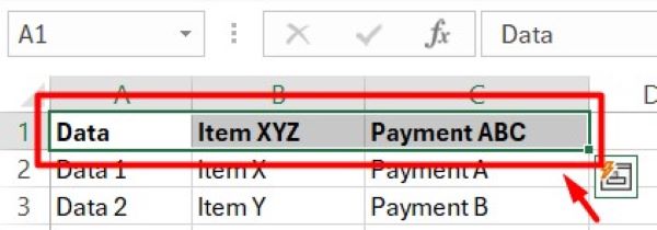
2. Access the filter tool in Excel.
Navigate to the “Data” tab in the Excel ribbon at the top of the screen. After that, locate and click on the “Filter” button. This will enable the filtering options for your selected data range.

3. Add filter arrows to the column headers.
Once you’ve clicked the “Filter” button, filter arrows will appear on the headers of each column in your selected data range. These arrows indicate that filtering is now available for those columns.

4. Customize how your filter criteria looks.
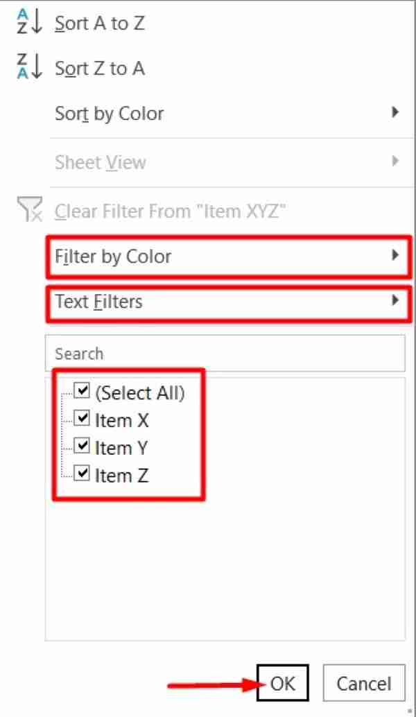
Click the dropdown arrows next to each column header to enable filtering. Select your filtering criteria from the menu, uncheck “Select All,” and check specific items to include. Additionally, explore further refinement options such as “Filter by Color” or “Text Filters,” then press “OK.”
5. Save the filter view to finalize your settings.
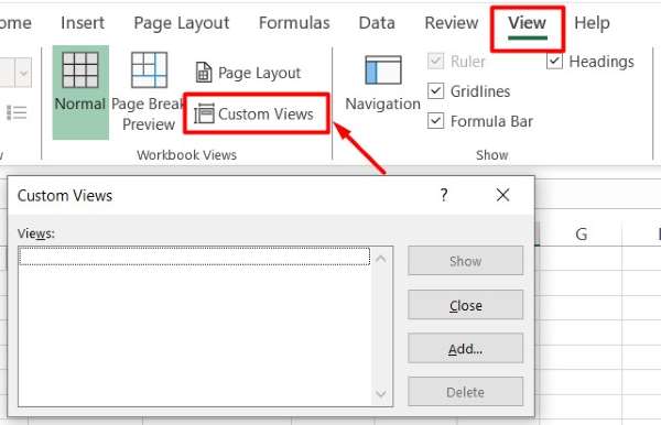
Afterward, save your filtered view by going to the “View” tab on the Excel ribbon and selecting “Custom Views” in the “Workbook Views” group.
6. Assign a name to your filtered view.
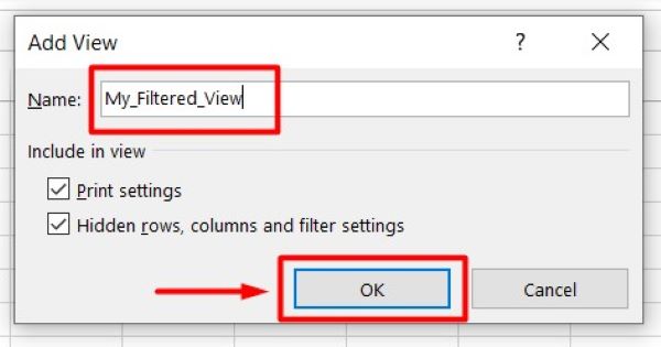
From the “Custom Views,” name your filtered view by clicking “Add.” Next, press “OK” to save it, as it ensures easy access to your customized view whenever needed.
7. Accessing and applying your saved filtered views.
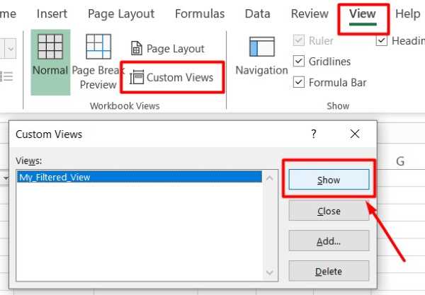
Whenever you want to retrieve your filtered data, return to the “View” tab and choose “Custom Views.” Then, select the view you saved earlier and click “Show” to apply it instantly, displaying your data precisely as you customized it.
We hope you now better understand how to save a FILTER in Excel. If you enjoyed this article, you might also like our article on how to use the FILTER and UNIQUE functions in Excel or our article on how to set up the Excel FILTER function with Wildcard.

