How to Split a Cell Diagonally in Excel And Fill Half With Color
In this article, we will show you how to split a cell diagonally in Excel and fill half with color. Simply follow the steps below.
Split a Cell Diagonally in Excel and Fill Half With Color
Follow the steps below to split a cell diagonally in Excel and fill half with color.
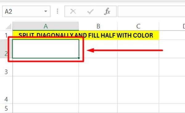
1. Select the Cell for Diagonal Split
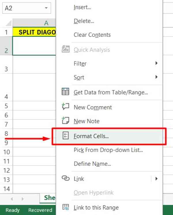
Click on the cell that you want to split diagonally. In our example, we will select A2. This cell will be the one where you apply the diagonal split and color fill. Make sure the cell is highlighted.
2. Right-Click the Cell and Choose Format Cells
Right-click on the selected cell to open a context menu. From this menu, choose “Format Cells” to open a dialog box with various formatting options for the cell.
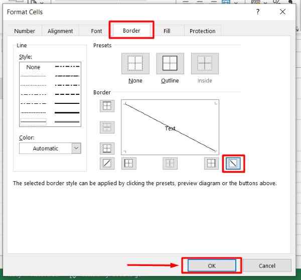
3. Add a Diagonal Line in the Border Tab
In the Format Cells dialog box, find and click on the “Border” tab. In the “Border” tab, click on the diagonal line button that goes from the bottom-left corner to the top-right corner of the cell. This action adds a diagonal line inside the selected cell. Click “OK” to apply the changes and close the dialog box.
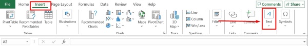
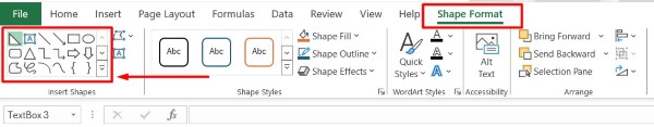
4. Insert Text Boxes in the Upper and Lower Halves
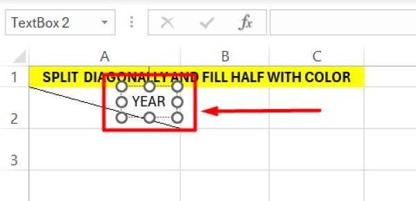
Go to the “Insert” tab on the ribbon at the top of Excel. Click on “Text Box,” then draw a small text box in the upper half of the diagonally split cell.
Type any text you need for the upper half. Repeat this step to add a text box in the lower half of the cell.
5. Format the Text Boxes
Adjust the sizes and positions of both text boxes so they fit neatly within their respective halves. Right-click on each text box, select “Format Shape,” and make any necessary formatting changes to the text inside.
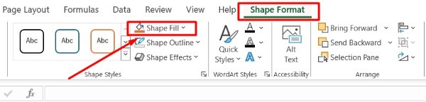
6. Fill the Upper Half with Color
Click on the text box in the upper half to select it. Go to the “Format” tab on the ribbon, click on “Shape Fill,” and choose the color you want to use for the upper half of the cell. This will fill the text box, and thus the upper half of the cell, with the chosen color.
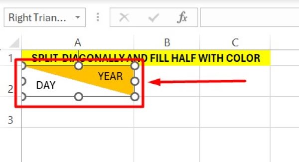
7. Fill the Lower Half with Color
Click on the text box in the lower half to select it. Go to the “Format” tab, click on “Shape Fill,” and select a color for the lower half of the cell. This will fill the text box, and thus the lower half of the cell, with the chosen color. Adjust the positions of the text boxes if necessary to ensure the text is legible and fits properly. Your cell is now split diagonally with each half filled with color.
We hope that you now better understand how to split a cell diagonally in Excel and fill half with color. If you enjoyed this article, you might also like our article on ways to split a single cell in Excel or our article on how to split screen in Excel.