How to Split Screen in Excel (Easiest Way in 2024)

In this article, we will show you how to split screen in Excel. Simply follow the steps below.

Split Screen in Excel

Follow the steps below on how to split screen in Excel.

1. Organize Your Data

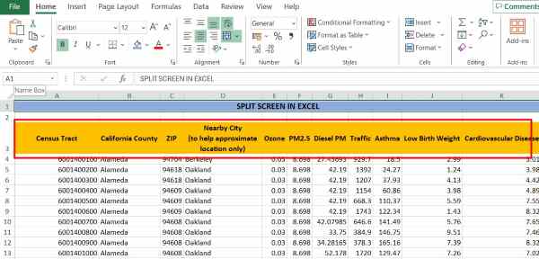
Arrange your data within the spreadsheet. This could involve typing in data, formatting cells, or importing data from another source. Ensure your data is structured in a way that makes sense for your analysis.

2. Access Viewing Options

At the top of the Excel window, find and click on the “View” tab. This will reveal options related to how your spreadsheet is displayed.

3. Activate Split Screen Mode

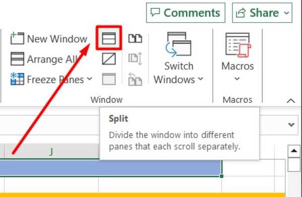
Within the “View” tab, locate the “Window” group. Click on the “Split” button. This action will divide your spreadsheet into separate panes, allowing you to view different sections simultaneously.

4. Fine-Tune the Split

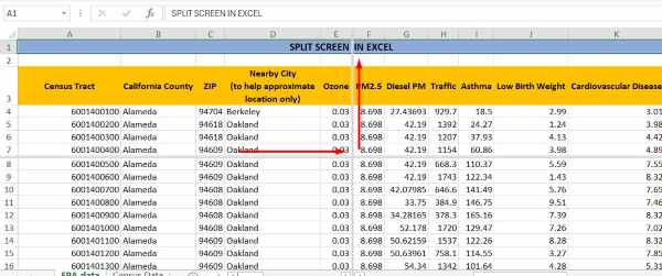
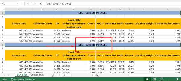
Adjust the split by dragging the split bar to your preferred location. This determines where the split between panes occurs, giving you control over what you see in each pane.

5. Navigate Through Panes

Once the split screen is activated, you can scroll through each pane independently. This allows you to view different parts of your spreadsheet simultaneously and navigate seamlessly through your data.

We hope you now have a better understanding of how to split screen in Excel. If you enjoyed this article, you might also like our article on ways to split a cell diagonally in Excel and fill half with color or our article on how to split multiple lines in one cell in Excel.