SUMIF Blank in Excel (How to Use It in 2024)

In this article, we will show you how to use the SUMIF blank in Excel. Simply follow the steps below.

SUMIF Blank in Excel

To sum blank values, you can use an empty string (“”) with the SUMIF function. This function is useful for large datasets as it helps identify blank cells and reveal data patterns or anomalies.

Syntax

Here’s the basic syntax for using SUMIF to sum values in cells that are blank:

=SUMIF(range, “”, sum_range)

where:

range: This is the range of cells that you want to evaluate for the blank condition.

“”: This is the criterion. In this case, it represents a blank cell.

sum_range: This is the range of cells from which you want to sum values based on the blank cells in the first range.

How to Use SUMIF Blank in Excel

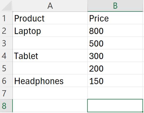
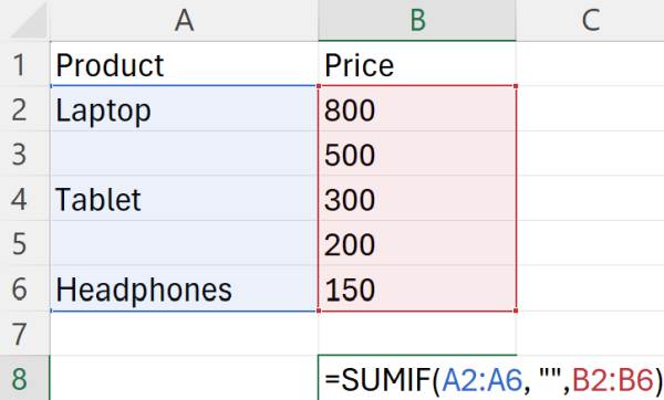
To use the SUMIF blank in Excel, we will work with a dataset containing product names in Column A and prices in Column B. Follow the steps below:

1. Choose the Cell for Calculating the Total Price

Decide where you want Excel to display the total price of products with blank quantities. In our case, let’s choose cell B8.

2. Use the SUMIF Formula to Calculate the Total Price

In cell B8, type the following formula:

=SUMIF(A2:A6, “”, B2:B6)

This formula tells Excel to sum up the prices (values in B2:B6) for products whose names (values in A2:A6) are blank or empty.

3. Press Enter to Calculate

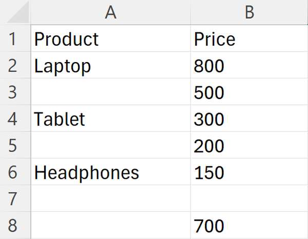
After entering the formula in cell B8, press the Enter key. Excel will process the formula and calculate the total price based on the specified conditions.

We hope that you now have a better understanding of how to use SUMIF Blank in Excel. If you enjoyed this article, you might also like our article about using SUMIF for cells that are not blank in Excel or our article on how to use Excel SUMIFS with wildcard.