SUMIF if Cell Contains Partial Text in Excel (Easiest Way in 2025)
In this article, we will show you how to create an Excel formula using SUMIF for a cell with partial text. Simply follow the steps below.
SUMIF Function in Excel
The SUMIF function in Excel allows you to sum values based on a criterion containing specific partial text by using wildcard characters. This function can help in summing up expenses, income, or other financial data based on categories, account names, or descriptions.
SUMIF Formula in Excel
The basic syntax for the SUMIF function in Excel is as follows:
=SUMIF(range, criteria, sum_range)
Where:
range: This is the range of cells that you evaluate with the criteria. Excel checks each cell in this range to see if it meets the criteria specified.
sum_range: It’s the actual range of cells to sum.
criteria: This defines the condition that must be met for a cell in the range to be included in the sum. Criteria can be a number, expression, cell reference, or text that defines which cells will be added. You can use wildcards like (*) and (?) for partial text matches.
The Asterisk wildcard (*) serves as a wildcard for any number of characters. If you want to sum values where the corresponding cells contain a specific substring, you can use * before and after your substring. For example:
=SUMIF(A1:A10, “*text*”, B1:B10)
In this formula, Excel sums the values in the range B1:B10 where the corresponding cells in A1:A10 contain the substring “text” anywhere.
On the other hand, the Question Mark (?) wildcard stands for any single character. For example, if you are looking for a specific pattern where one character might vary, you could use:
=SUMIF(A1:A10, “te?t”, B1:B10)
This formula would sum the values in B1:B10 where the corresponding cells in A1:A10 have “text,” “tent,” “test,” etc., with any single character replacing the question mark.
These approaches are useful when you need to sum values based on cells containing specific text patterns in another range.
How to Use the Excel SUMIF for a Cell That Contains Partial Text
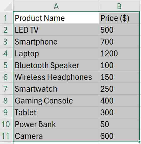
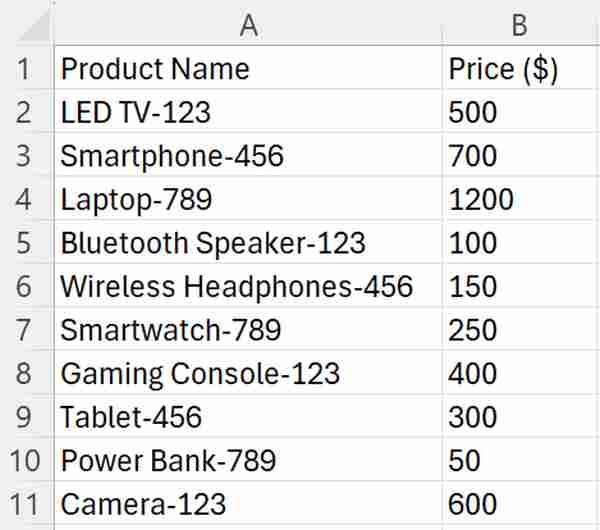
To learn how to use Excel’s SUMIF function for cells containing partial text, we will use a dataset that contains the product name in Column A and the prices in Column B. Follow the steps below:
1. Choose the Range Containing Product Names and Prices
Begin by selecting the cells that contain the product names and their respective prices. This means clicking and dragging your cursor over the cells. In our example, the range we’ll use is A2:B11, where column A contains the product names and column B contains their prices.
2. Determine the Partial Text to Find
Think about the specific part of the product names that you want to search for. For instance, if you’re interested in products related to “phones,” you’ll be searching for names that include this term.
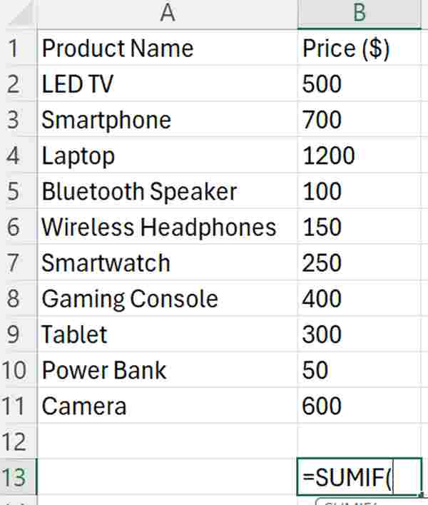
3. Begin Writing Your SUMIF Formula
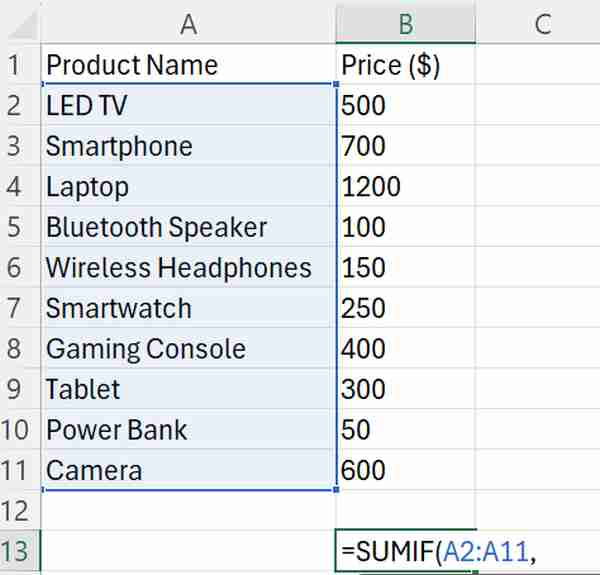
In the cell where you want the total price to appear, start typing =SUMIF( to initiate the formula that will help us find and sum values based on partial text matches. In our case, let’s use B13.
4. Specify the Range to Search for Partial Text
After =SUMIF(, enter the range where you want Excel to search for the partial text. In our case, we’re looking at the product names (A2:A11) to find matches.
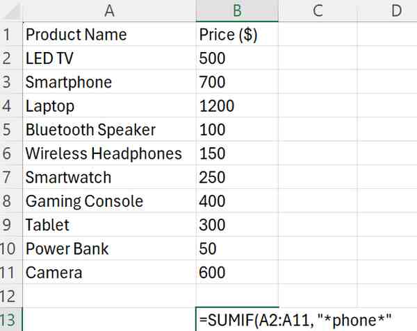
5. Include the Partial Text Using Wildcards
After the first comma in the formula, input “*phone*” to instruct Excel to find products with “phone” in their names. The asterisks (*) before and after “phone” allow for any text before or after it, giving us flexibility in matching.
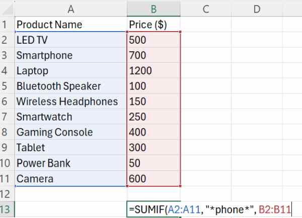
6. Define the Range to Sum Based on the Partial Text
After the second comma in the formula, specify the range of prices (B2:B11) that you want to sum based on the partial text match. This tells Excel which prices to add up when a match is found.
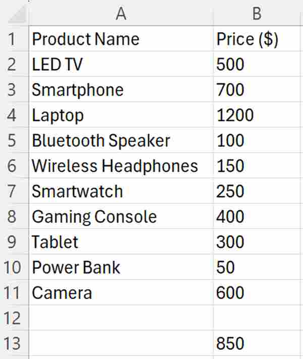
7. Complete the Formula
Close the formula with a closing parenthesis ) and press Enter. Excel will then calculate and display the total price of products containing “phone” in their names.
Using Excel SUMIF for Cells That Contain Text and Numbers
To use SUMIF for cells that contain text and numbers, you can wildcard characters. Here’s how to do it:
1. Define Criteria for Summing
Clearly define the criteria for summing the values. In this example, we aim to sum values based on cells in Column A that contain “456” in their text.
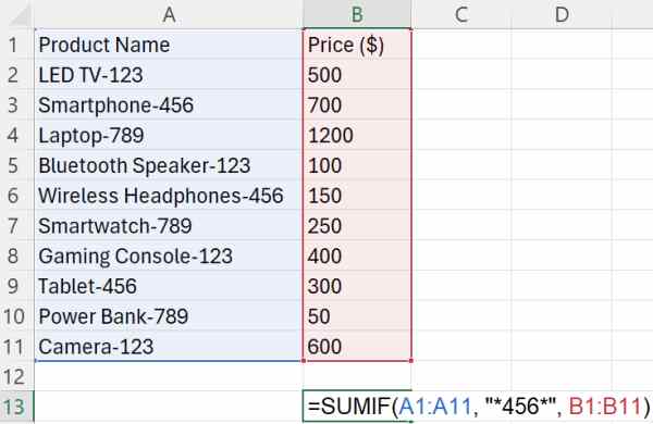
2. Set Up the SUMIF Formulas
To sum values based on the criteria, use the SUMIF function. For cells containing “456” in the text, write the formula:
=SUMIF(A:A, “*456*”, B:B)
3. Apply the Formulas
Place the formula in the cell where you want the sum to appear. For our example, we’ll use cell B13 as the destination for the sum. Type in the following formula: =SUMIF(A1:A11, “*456*”, B1:B11).
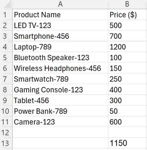
4. Calculate and Verify Results
Press Enter after entering the formula to calculate and verify the sums. Excel will display the total price of the products that contain “phone” in their names in the cells where you entered the formulas.
We hope you now have a better understanding of how to use SUMIF for a cell that contains partial text in Excel. If you enjoyed this article, you might also like our article on how to sum dates in Excel or our article on how to remove column letters and row numbers in Excel when printing.