SUMIF Not Blank in Excel (How to Use it in 2025)
In this article, you will learn how to use SUMIF not blank in Excel. Simply follow the steps below.
SUMIF Not Blank in Excel
The SUMIF function in Excel allows you to sum values in a range based on a specific condition. To sum only the non-blank cells in a range, use the SUMIF function along with the “<>” operator, which means “not equal to.”
Syntax
Here’s the general syntax for using SUMIF to sum values in cells that are not blank:
=SUMIF(range, criteria, [sum_range])
range: This is the range of cells that you want to evaluate using the criteria.
criteria: This is the condition that you want to apply to the cells in the range.
sum_range: This is the actual range of cells that you want to sum.
How to Use SUMIFS Not Blank in Excel
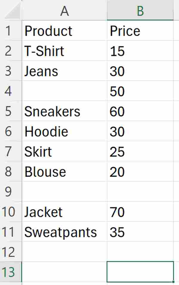
To use the Excel SUMIF not blank function, we will work with a dataset containing product names in Column A and prices in Column B. Follow the steps below:
1. Choose a Destination Cell for Total Price Calculation
Select an empty cell where you want the total price to appear. Let’s say we choose cell B13.
2. Use SUMIF to Calculate the Total Price
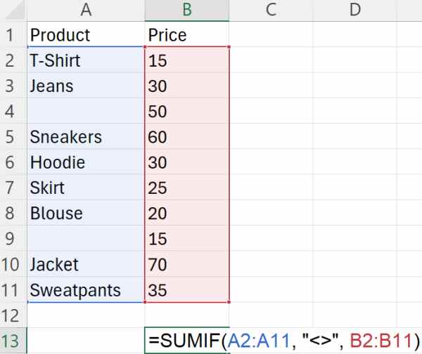
In cell B13, type the following formula:
=SUMIF(A2:A11, “<>”, B2:B11)
This formula tells Excel to add up the prices of all items listed in the Category column that are not blank.
3. Press Enter to Calculate
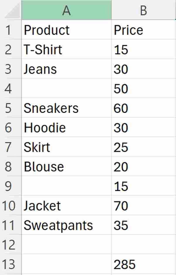
After typing the formula, hit the Enter key. Excel will then compute and display the total price of all items that are not blank.
We hope that you now have a better understanding of how to use SUMIF not blank in Excel. If you enjoyed this article, you might also like our article about using Excel SUMIF not equal to function or our article on how to use Excel SUMIF for blank cells.

