Filter by Color in Excel (Easiest Way in 2025)
In this article, we will show you exactly how to filter by color in Excel. Simply follow the steps below.
How to Filter by Color in Excel
To filter by color in Excel, simply follow the process below.
1. Select the Column or Data Range to Filter
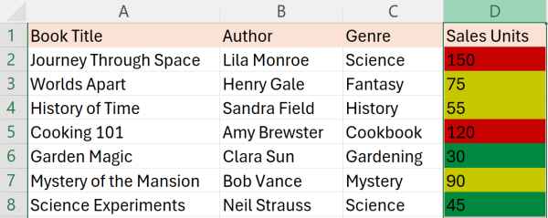
In our example, we have a dataset from a school book fair that lists various books from cells A2 to A8, each with their respective sales figures in cells D2 to D8.
These sales units are color-coded to visually represent their sales performance:
Red for Sales Units >= 100 (Bestsellers)
Yellow for Sales Units between 50 and 99 (Average sellers)
Green for Sales Units < 50 (Low sellers)
Your task is to filter this data by color to quickly identify books in each sales category.
To begin filtering, click at the top of the ‘Sales Units’ column to select it.
2. Activate the Filter Function from the Data Tab
Navigate to the ‘Data’ tab located in the Ribbon at the top of Excel. Here, you’ll find the ‘Filter’ button. Click this button to enable dropdown arrows on each column header within your selected range.

3. Apply the Color Filter to the ‘Sales Units’ Column
Click on the dropdown arrow in the ‘Sales Units’ column header to access the filtering options. Look for the ‘Filter by Color’ option within the menu. Hover over it, and then select the color you want to filter by—choose Red to see all bestsellers, Yellow for average sellers, or Green for low sellers. In our case, let’s choose the color yellow.

4. Check the Filtered Results to Ensure Accuracy
After applying the color filter, your Excel sheet will now display only the rows that are highlighted in Yellow, corresponding to average sellers.

Filter by Multiple Colors in Excel
To filter by multiple colors in Excel, we will work with the same dataset from our previous example that contains each book’s sales performance. Red represents bestsellers, Yellow denotes average sellers, and Green signifies low sellers. Follow the steps below:
1. Place a Helper Column
Next to the ‘Sales Units’ column, add a new column and name it “Sales Performance”. This column will be used to identify sales categories based on color, assisting in the filtering process.

2. Insert an ‘IF’ Formula to Categorize Sales Automatically
Click on the first cell in the ‘Sales Performance’ column next to your ‘Sales Units’. In our example, E2 is the first row in our sales performance column and our sales data begins in cell D2.
In E2, enter the following formula:
=IF(D2>=100, “Bestseller”, IF(D2>=50, “Average”, “Low”))
This formula checks:
If the sales in D2 are 100 or more, it labels it as “Bestseller”.
If the sales are 50 to 99, it labels it as “Average”.
If the sales are less than 50, it labels it as “Low”.

3. Drag the Formula Down
After entering the formula in E2, position your cursor at the fill handle at the bottom-right corner of the cell.

Then, click and drag it down through the column to apply the formula to the other cells in the ‘Sales Performance’ column.

4. Apply Filters Based on Formula Results
Click on the ‘Sales Performance’ header and go to the Data tab. Then, click on Filter.

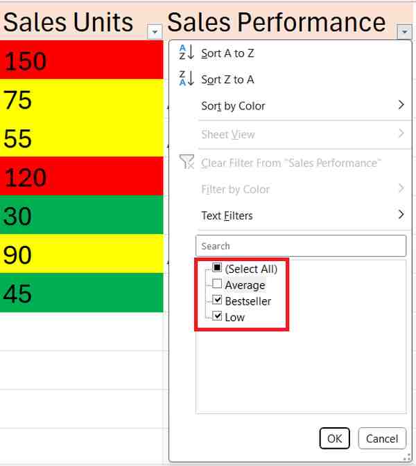
Click the dropdown arrow in the ‘Sales Performance’ column header. From the menu, select the checkboxes next to the performance labels you are interested in (e.g., “Bestseller”, “Average”, “Low”). This will filter the rows in your spreadsheet to only show those that meet your selected criteria. In our case, let’s choose both the “Bestseller” and “Low”.
5. Review the Filtered Data
With the filters applied, your Excel sheet will now display only those books that match the selected sales performance categories.

Filter by Color Not Working in Excel
In order to fix the filter by color in Excel, simply follow the steps below.
1. Activate Data Filtering
Ensure that data filtering is active for your worksheet to apply a color filter. To do this, navigate to the “Data” tab in the file menu. Look for the ‘Filter’ button and click on it. This action turns on filtering for all the columns in your dataset, which is necessary for subsequent filtering steps.

2. Verify Manual Coloring of Cells
Confirm that the filter column in your data set is colored manually or through standard formatting. In our data set this in the Sales Units column.

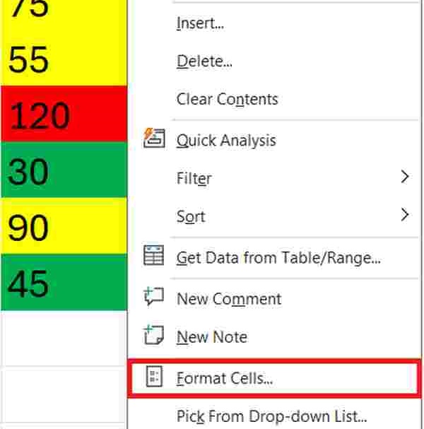
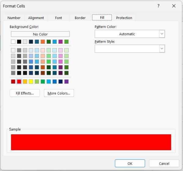
Right-click on one of the colored cells in the column, and choose ‘Format Cells’ from the context menu.
In the format cells window, click the ‘Fill’ tab to verify if the color was applied directly here rather than through conditional formatting.
3. Apply a Color Filter
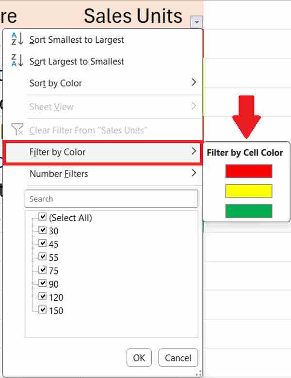
Initiate color filtering by clicking on the filter dropdown arrow in the header of your filter column. In our example, this is the ‘Sales Units’ Column.
From the dropdown menu, select ‘Filter by Color,’ then choose the specific color you wish to filter by. This selection filters the data to display only those rows that match the color of the cell you selected.
4. Clear and Reapply Filters
If your initial attempt to filter by color does not work, it may be necessary to reset the filters. Go to the “Data” tab in the file menu and click on the ‘Clear’ button to remove all active filters. After clearing, reactivate the filters and attempt to apply the color filter again to ensure that all settings are correctly recognized and applied.

5. Ensure Excel Version Supports Color Filtering
Check that your version of Excel supports the filter-by-color feature. This is generally available in Microsoft Excel 2007 and newer versions. If you’re using an older version, this feature might not be available, which could be why the color filtering is not working.
6. Access Excel Help for Further Assistance
If you’re still facing difficulties with filtering by color, Excel’s Help system can provide more detailed assistance. You can access it by pressing ‘F1’ or by selecting ‘Help’ from the Ribbon. Once in the Help interface, search for “filter by color” for targeted help articles and troubleshooting tips specific to your version of Excel.

We hope that you now have a better understanding of how to filter by color in Excel. If you enjoyed this article, you might also like our article on how to filter dates in Excel or our article on how to filter bold text in Excel.

