How to Freeze a Formula in Excel (Easiest Way in 2025)
In this article, we will show you how to freeze a formula in Excel. Simply follow the steps below.
Freeze a Formula in Excel
Follow the steps below on how to freeze a formula in Excel.
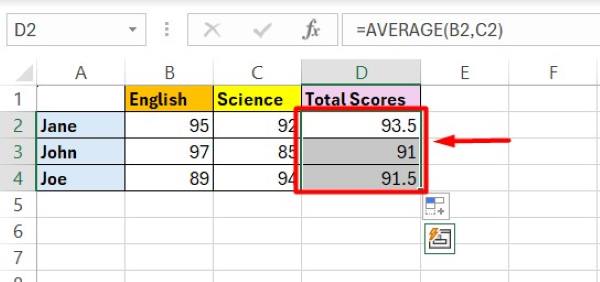
1. Select the Cell Containing the Formula
Click on the cell that contains the formula you want to freeze. This will highlight the cell and display the formula in the formula bar at the top of the Excel window. Make sure the cell is selected and you can see the formula clearly.
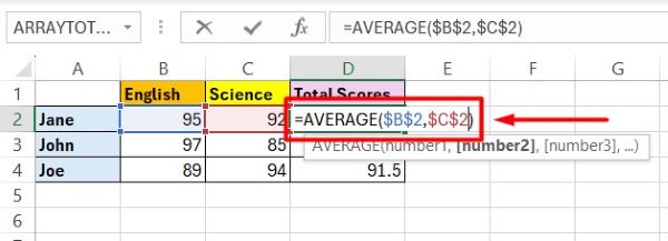
2. Enter Edit Mode for the Selected Cell
Double-click the selected cell or press F2 on your keyboard. This will switch the cell into edit mode which allows you to modify the formula directly within the cell. You should now see a blinking cursor in the cell, ready for you to make changes.
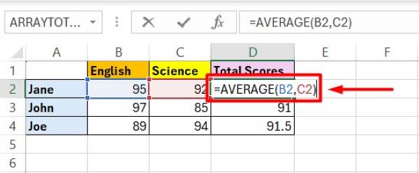
3. Add Dollar Signs to Make Cell References Absolute
In the formula, find the cell references (e.g., B2). Add a dollar sign ($) before both the column letter and the row number of each cell reference you want to freeze. For example, change B2 to $B$2. This ensures the cell reference remains constant, even when you copy the formula to other cells. Repeat this for all cell references you want to freeze within the formula.
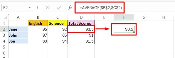
4. Press Enter to Confirm the Changes
After adding the dollar signs to the cell references, press Enter on your keyboard. This will exit edit mode and apply the changes to the formula. Now, when you copy and paste this formula to other cells, the references will remain absolute and won’t change.
We hope that you now have a better understanding of how to freeze a formula in Excel. If you enjoyed this article, you might also like our article on how to freeze selected columns in Excel or our article on ways to freeze horizontal and vertical panes Excel.