How to Freeze Horizontal and Vertical Panes in Excel (2024)

In this article, we will show you how to freeze horizontal and vertical panes in Excel. Simply follow the steps below.

Freeze Horizontal and Vertical Panes Excel 

Follow the steps below on how to freeze vertical and horizontal panes in Excel.

1. Select the Cell Below and to the Right of the Desired Freeze Point

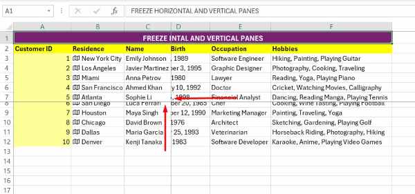
Click on the cell that is directly below the row you want to freeze and to the right of the column you want to freeze. In the example below, we will select cell D8.

2. Go to the View Tab in the Ribbon

Look at the top of your Excel window. You will see several tabs, such as “Home,” “Insert,” and “Page Layout.” Click on the “View” tab to access view-related options.

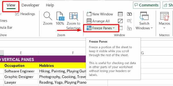
3. Click on the Freeze Panes Button in the View Tab

In the “View” tab, locate the “Window” group. Within this group, find and click on the “Freeze Panes” button. This button will display a drop-down menu with different freezing options.

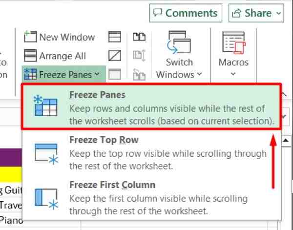
4. Select the Freeze Panes Option from the Dropdown

In the drop-down menu that appears when you click “Freeze Panes,” select the “Freeze Panes” option. This option will freeze the rows above and the columns to the left of the cell you selected in step 1. For example, if you selected cell B2, row 1 and column A will be frozen.

5. Scroll to Verify that Rows and Columns are Frozen

Scroll through your worksheet to check if the panes are correctly frozen. The rows and columns you wanted to keep visible should remain in place while you scroll through other parts of the worksheet. For example, if you froze the top row and the first column, they should stay visible as you scroll down or to the right.

We hope you now have a better understanding of how to freeze horizontal and vertical panes in Excel. If you enjoy this article, you might also like our article on how to freeze a formula in Excel or our article on how to freeze tabs in Excel.