How to Freeze Selected Rows in Excel (Easiest Way in 2024)

In this article, we will show you how to freeze selected rows in Excel. Simply follow the steps below.

How to Freeze Specific Rows in Excel

Below, we outline the steps to freeze specific rows in Excel.

1. Identify the Selected Rows You Want to Freeze

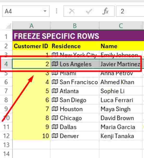
Before proceeding, identify the specific rows in your spreadsheet that you want to stay in place as you navigate through your data. To do this, click and drag to select the rows you wish to freeze. In our example below, we will freeze the fourth row.

2. Access the “View” Tab

To access the necessary settings, locate and click on the “View” tab situated at the top of the Excel window. This tab provides various options related to the visual display of your spreadsheet.

3. Find the “Freeze Panes” Option

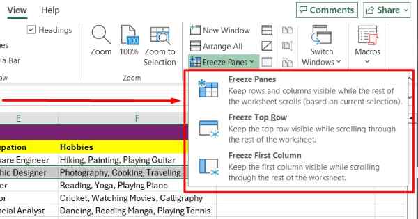
Within the “View” tab, find the “Window” group. Inside this group, you’ll see the “Freeze Panes” option. Click on it to reveal further options related to freezing rows and columns.

4. Select the Appropriate Freezing Option

After clicking on “Freeze Panes,” a dropdown menu will appear with three choices: “Freeze Panes,” “Freeze Top Row,” and “Freeze First Column.” If you want to freeze a selected row, ensure to select the row below the specified row before choosing the appropriate option.

5. Confirm the Freezing Effect of the Selected Rows

Once you’ve selected the freezing option, scroll down your spreadsheet to verify that the chosen rows remain visible at the top, unaffected by your scrolling actions. This ensures that the freezing feature is working correctly and that the desired rows are indeed frozen in place.

We hope you now better understand how to freeze selected rows in Excel. If you enjoyed this article, you might also like our article on how to freeze the header in Excel or our article on how to freeze specific columns in Excel.