How to Freeze a Tab in Excel (Easiest Way in 2024)

In this article, we will show you how to freeze a tab in Excel. Simply follow the steps below.

How to Freeze Tabs in Excel 

Follow the steps below on how to freeze tabs in Excel.

1. Open the “View” Tab in the Excel Menu

Click on the “View” tab in the top menu. This tab contains options for adjusting how you view your spreadsheet. The “View” tab is usually located between the “Review” and “Help” tabs.

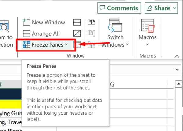
2. Click the “Freeze Panes” Button in the View Tab

In the “View” tab, locate the “Freeze Panes” option. Click the “Freeze Panes” button to open a dropdown menu with more options for freezing rows and columns.

3. Select “Freeze Top Row” to Keep the Top Row Visible

To keep the top row visible while you scroll down the spreadsheet, select “Freeze Top Row” from the dropdown menu.

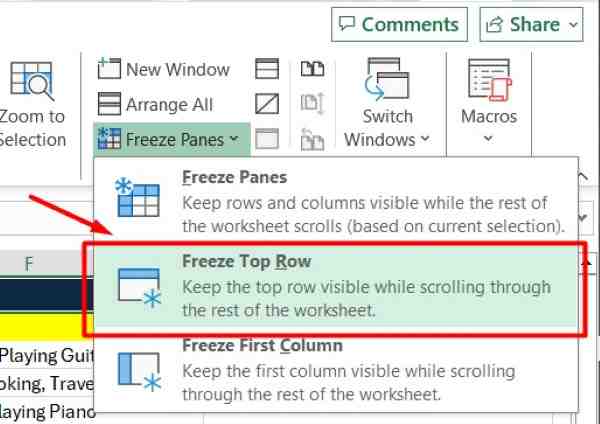
This option will ensure that the top row remains static and visible no matter how far you scroll down. In our example below, we will freeze row 1.

4. Select “Freeze First Column” to Keep the First Column Visible

To keep the first column visible while you scroll across the spreadsheet, select “Freeze First Column” from the dropdown menu.  

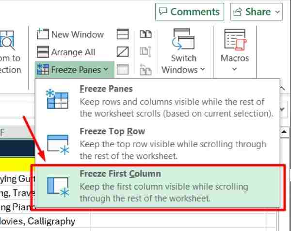
This option will ensure that the first column remains static and visible no matter how far you scroll to the right.

5. Use “Freeze Panes” to Freeze Specific Rows and Columns

If you need to freeze both specific rows and columns, select “Freeze Panes” from the dropdown menu.  

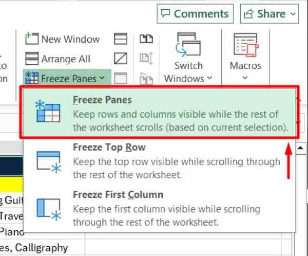
Click on the cell below and to the right of the rows and columns you want to keep visible. This will freeze all rows above and columns to the left of the selected cell. In the example below, we selected cell C7.

We hope that you now have a better understanding of how to freeze a tab in Excel. If you enjoy this article, you might also like our article on ways to freeze vertical and horizontal panes in Excel or ways to fix freezes when copying and pasting in Excel.