Highlight Blank Cells in Excel (Easiest Way in 2025)
In this article, we will show you how to highlight blank cells in Excel. Simply follow the steps below.
How to Highlight Blank Cells in Excel Using Conditional Formatting
Below, we outline the steps on how to highlight blank cells in Excel using conditional formatting.
1. Select the Range to Highlight
Identify the specific range of cells where you want to highlight any blank entries. In our example below, we highlighted the first and last names.

2. Navigate to Conditional Formatting
Go to the “Home” tab in Excel. Look for the “Styles” group, typically found in the upper ribbon of the Excel window.

3. Access Conditional Formatting Options
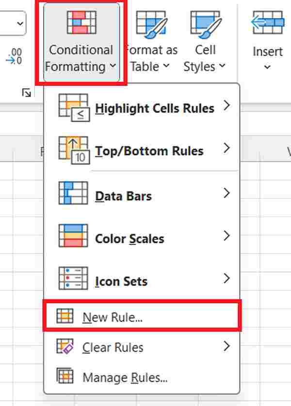
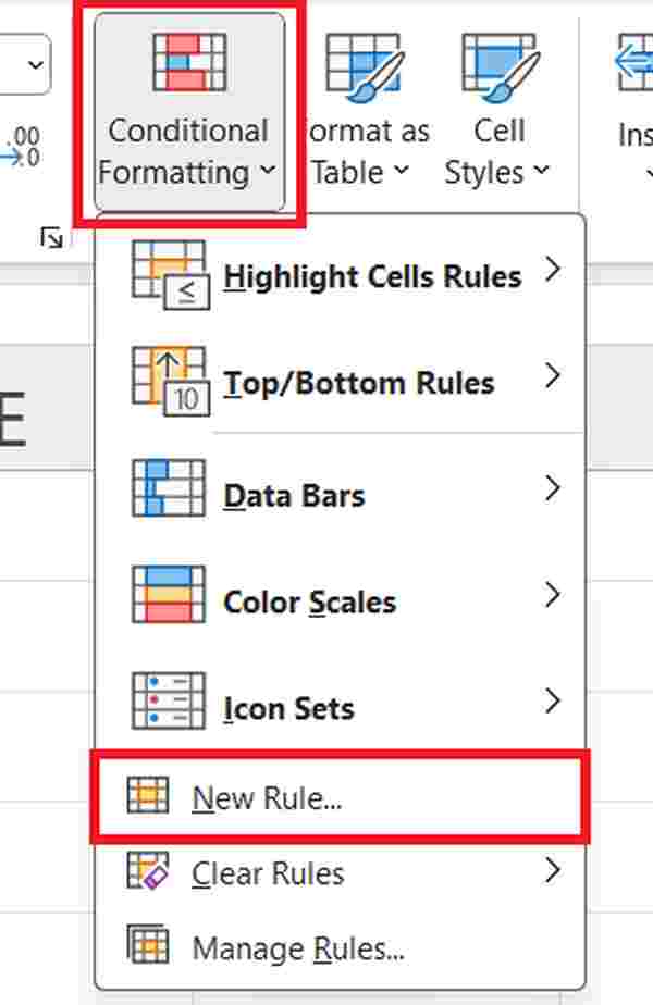
Within the “Styles” group, locate and click on “Conditional Formatting.” This action will prompt a dropdown menu with various formatting options. Then, from the dropdown menu, choose “New Rule.” This selection will open a new dialog box where you can define the formatting rule.
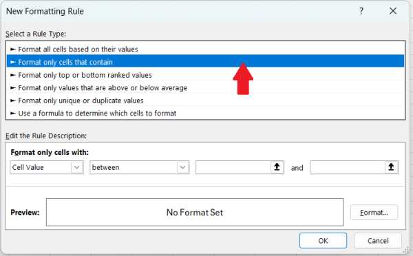
4. Choose “Format Only Cells That Contain”
In the new dialog box, you’ll see a list of rule types. Select “Format only cells that contain” to specify the condition for applying your formatting.
5. Specify the Condition for Blank Cells
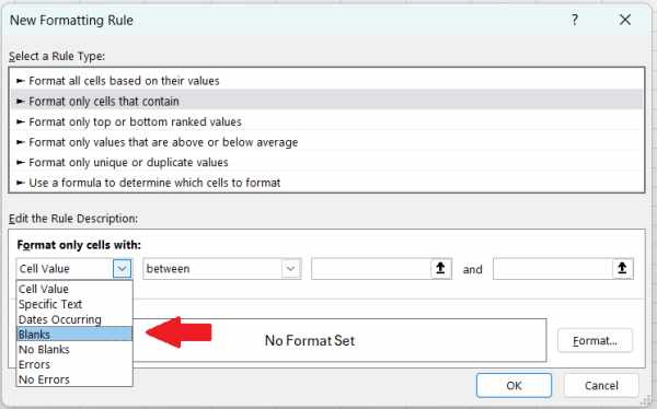
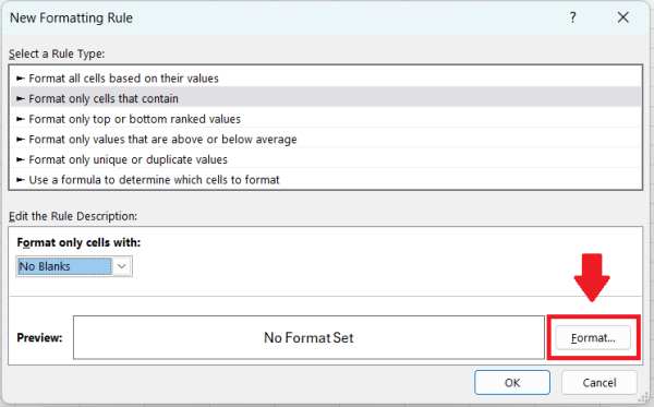
After selecting the rule type, move on to defining the condition. Choose “Blanks” from the dropdown menu under the rule settings. This tells Excel to identify and format cells that are empty.
6. Define Formatting for Blank Cells
To determine how Excel should visually represent blank cells, click on the “Format” button. This action will open the “Format Cells” dialog box, where you can set the desired formatting style.
7. Apply the Formatting Style
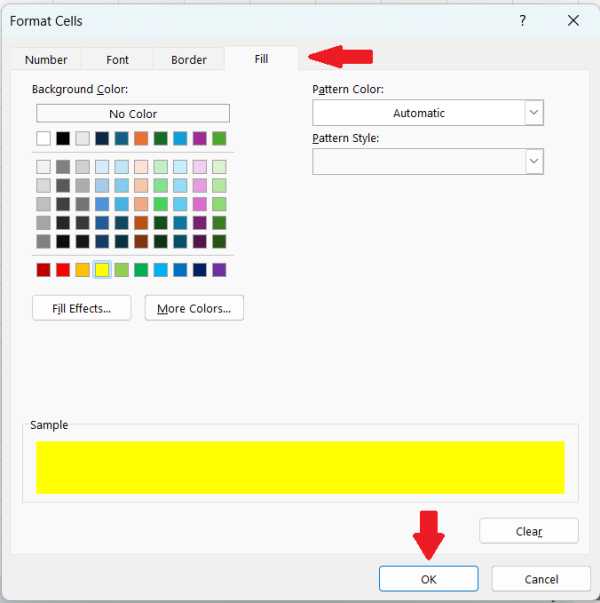
In the “Format Cells” dialog box, navigate to the “Fill” tab. Here, choose the background color or any other formatting options you want for highlighting the blank cells. In our case, let’s choose the color yellow under the “Fill” tab as the fill color for cells with blank first names. Once done, click “OK” to confirm your choices.
8. Preview and Confirm the Formatting
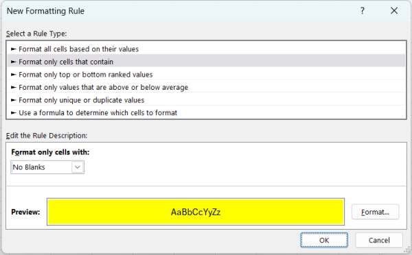
Back in the “New Formatting Rule” dialog box, review the preview section. This preview shows how Excel will format the blank cells based on your defined rule. Ensure the formatting appears as desired before proceeding. Once you’re satisfied with the preview, click “OK” in the “New Formatting Rule” dialog box to apply the rule.
9. View Results
Excel will now highlight the blank cells in the selected range according to your specified formatting.

Highlight Blank Cells in Excel Using Conditional Formatting Formula
To highlight blanks in Excel, you can use the ISBLANK function. Here’s how you do it:
1. Select the Range to Highlight
In our example below, click and drag your mouse to select the entire range of cells that includes the first and last names (B2:C6). Ensure you’ve selected all relevant cells to apply the formatting accurately.

2. Access Conditional Formatting
Navigate to the “Home” tab located at the top of Excel. This is where you’ll find the tools and options for formatting your data.

3. Initiate a New Conditional Formatting Rule
Under the “Conditional Formatting” dropdown menu within the “Home” tab, select “New Rule.” This action will open a dialog box where you can define the formatting rule.
4. Choose the Formula Option
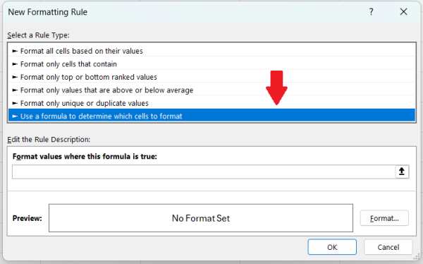
In the “New Formatting Rule” dialog box, opt for “Use a formula to determine which cells to format.” This choice allows you to specify conditions based on formulas.
5. Define the Formula for Blank Names
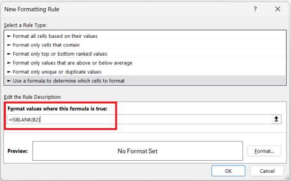
Enter the formula `=ISBLANK(B2)` in the formula box. This formula checks if the cell in the first name column (our reference starts from cell B2) is blank. Adjust the cell reference as needed based on your data.
6. Format Blank Names
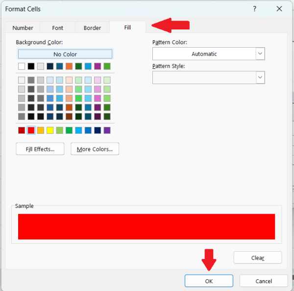
Click on the “Format” button within the “New Formatting Rule” dialog box. Here, you can choose the formatting style for cells with blank first names, such as fill color or font color changes. In our case, let’s choose the color red under the “Fill” tab as the fill color for cells with blank first names.
After selecting your desired formatting options, click “OK” to apply the formatting specifically to cells where the first name is blank
7. Blank Cells Are Highlighted
The selected cells should now be visually distinguished based on the formatting options you specified.

How to Highlight Blank Cells in Excel using Go To Special
Follow the steps below to highlight blank cells in Excel using the Go To Special function.
1. Select the Range of Cells Containing Your Data
Select every cell where you want to highlight blank entries. This step is crucial as it defines the area where Excel will apply the highlighting.

2. Open the “Go To Special” Dialog Box
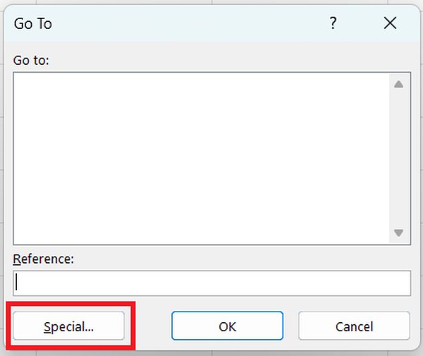
You can open the Go To Special Dialog Box using a keyboard shortcut. Press either `Ctrl + G` or `F5` on your keyboard. This action will bring up the “Go To” dialog box. From there, click on the “Special…” button.
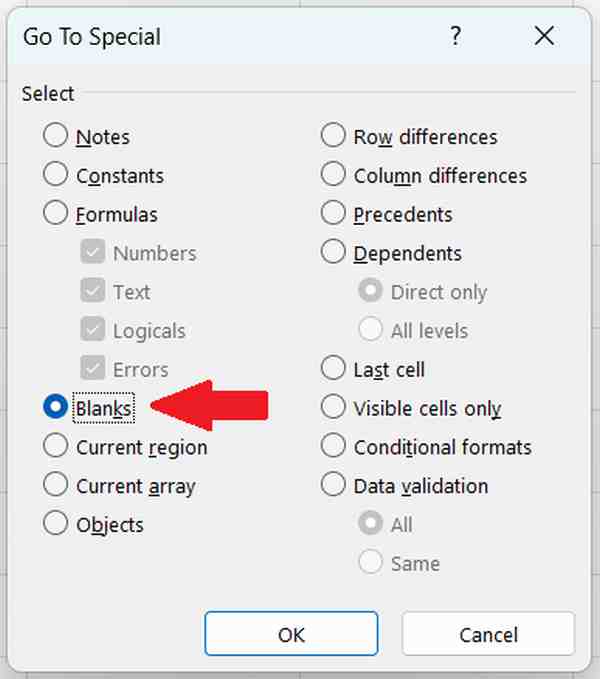
3. Choose the “Blanks” Option
In the “Go To Special” dialog box, you’ll see a range of options. Check the box next to “Blanks” and then click “OK.” This action instructs Excel to select all the blank cells within the range you specified earlier.
4. Apply Highlighting to Blank Cells
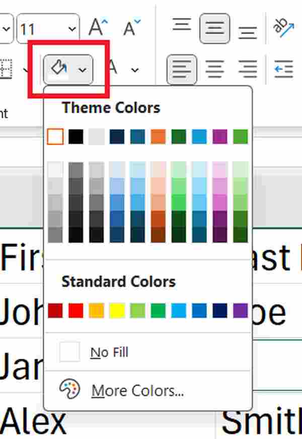
With the blank cells now selected, it’s time to apply the highlighting. Move to the “Home” tab in Excel. Locate the “Fill Color” option within the “Font” group and click on it. A color palette will appear. Choose a color that you want to use to highlight the blank cells. In our case, let’s choose the color yellow.
5. See Highlighted Blank Cells
The highlighted cells will now stand out, making it easier for you to identify and work with them.

We hope that you now have a better understanding of how to highlight blank cells in Excel. If you enjoyed this article, you might also like our article on how to delete duplicates in Excel or our article on how to highlight specific words in Excel.

