How to Highlight Highest Value in Excel (Easiest Way in 2025)
In this article, we will show you how to highlight the highest value in Excel. Simply follow the steps below.
Highlight Highest Value in Each Row in Excel
Follow the steps below on how to highlight the highest value in Excel.
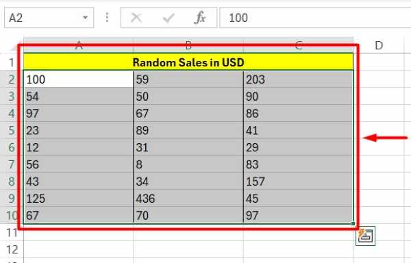
1. Select the Range of Cells Containing Your Data
Select the range of cells that contains the data you want to analyze. Click and drag your mouse to highlight all the relevant cells. This tells Excel which cells to consider when finding the highest value.
2. Navigate to the Conditional Formatting Menu
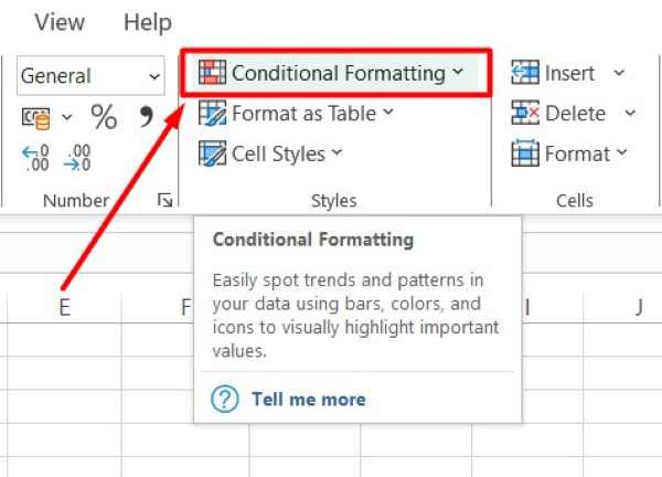
Go to the “Home” tab on the Excel ribbon. In the “Styles” group, click on “Conditional Formatting.” This opens a menu where you can create rules for formatting cells based on their values.
3. Start Creating a New Formatting Rule
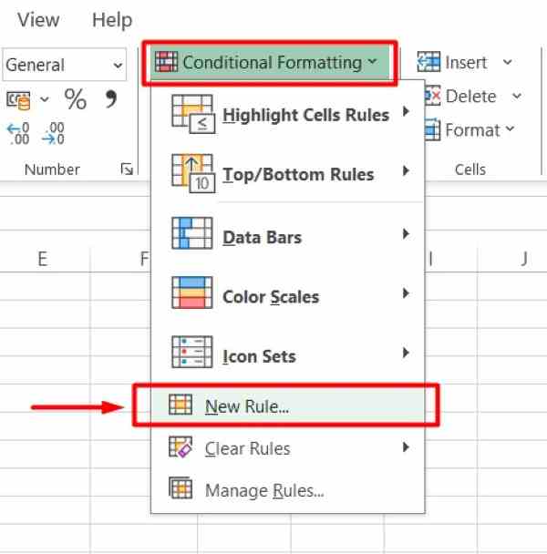
From the Conditional Formatting menu, click on “New Rule.” This option allows you to define a custom rule for highlighting cells according to specific criteria.
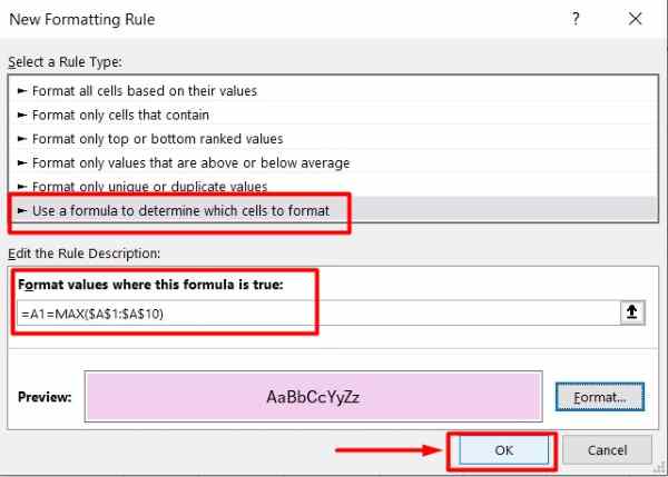
4. Choose to Use a Formula for Formatting
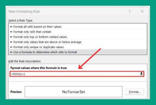
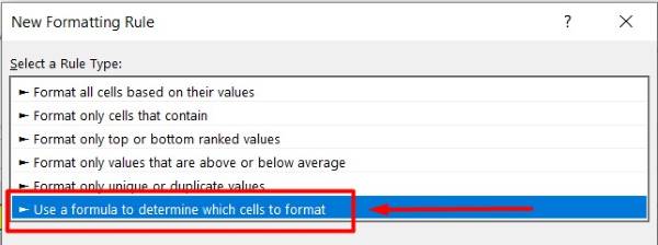
In the New Rule window, select “Use a formula to determine which cells to format.” This option lets you use a custom formula to decide which cells should be formatted based on your criteria.
5. Enter a Formula to Identify the Highest Value
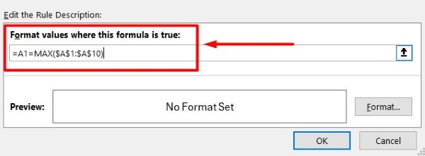
In the formula box, enter `=A1=MAX($A$2:$A$10)`, replacing `A1` and `$A$1:$A$10` with the appropriate cell references for your data range. Additionally, this should be applied to the rest of the columns such as `B1` or `C1`. This formula will check each cell to see if it contains the highest value in the specified range.
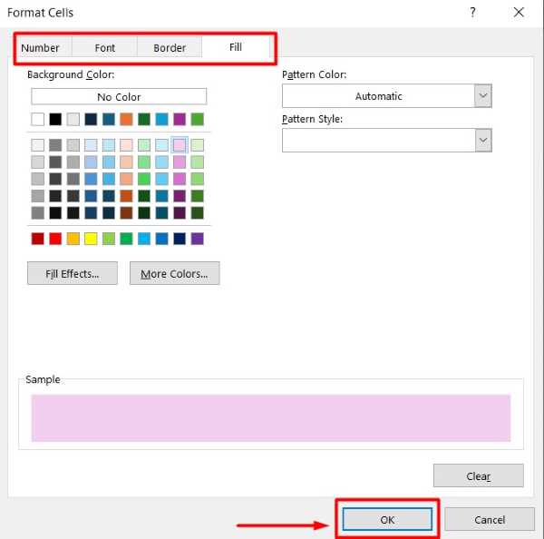
6. Define the Formatting for the Highest Value
Click on the “Format” button. In the Format Cells dialog box, choose the formatting options you want to apply to the highest value. This could be a specific fill color, font color, or border style. Click “OK” to confirm your choices.
7. Confirm and Apply the New Rule
After setting up the formula and formatting, click “OK” to apply the rule. Your selected cell range will now automatically highlight the cell with the highest value using the formatting you specified.
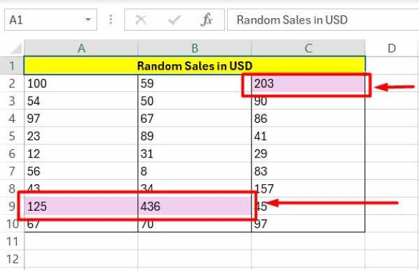
8. Check and Adjust the Highlighted Result
Review your data range to ensure the highest value is highlighted correctly. If necessary, adjust the cell references in the formula or modify the formatting settings to achieve the desired result.
We hope that you now have a better understanding of how to highlight the highest value in Excel. If you enjoy this article, you might also like our article on ways to compare two columns in Excel and highlight matches or our articles on how to highlight changes in Excel.