How to Freeze the Second Column in Excel (Easiest Way in 2025)
In this article, we will show you how to freeze the second column in Excel. Simply follow the steps below.
Freeze Second Column in Excel
Follow the steps below on how to freeze the second column in Excel.
1. Identify the Second Column to Freeze
Ensure the spreadsheet you want to work on is active. This is where you will apply the freezing action. Look at your spreadsheet and locate the second column. This is the column you want to remain visible at all times even when you scroll to the right.

2. Click on a Cell in the Third Column
Move your cursor to the third column and click on any cell within it. Freezing panes in Excel works to the left of the selected cell, so by clicking in the third column (Column C), you will keep the second column (Column B) fixed in place.

3. Navigate to the “View” Tab in the Menu
At the top of your Excel window, find and click on the “View” tab. This tab includes options that allow you to customize how you see and navigate your spreadsheet.

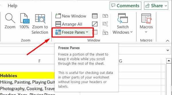
4. Click on “Freeze Panes” in the “View” Tab
Within the “View” tab, locate the “Freeze Panes” button. It is usually found in the “Window” section. Click on this button to open a dropdown menu with freezing options.
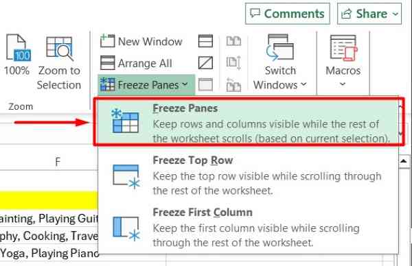
5. Select “Freeze Panes” from the Dropdown Menu
From the dropdown menu that appears, choose the “Freeze Panes” option. This will freeze all columns to the left of your selected cell in order to ensure the second column remains visible as you scroll horizontally.
6. Confirm the Second Column is Frozen
To verify that the second column is frozen, scroll horizontally in your spreadsheet. If the second column stays fixed while the rest of the columns move, the freezing action is successful.

We hope that you now have a better understanding of how to freeze a tab in Excel. If you enjoyed this article, you might also like our article on ways to fix freezing when copying and pasting in Excel or our article on how to freeze the second row in Excel.

