How to Hide Duplicates in Excel (Easiest Way in 2025)
In this article, we will show you how to hide duplicates in Excel. Simply follow the steps below.
Hide Duplicates in Excel
Duplicate data in Excel can be hidden using two methods: ‘Conditional Formatting’ and ‘Advanced Filter’. We will discuss how to use each method in the following sections.
Method 1: Using Conditional Formatting to Hide Duplicates
Below, we outline the steps on how to hide duplicates in Excel using Conditional Formatting.
1. Highlight the Data You Want to Check for Duplicates
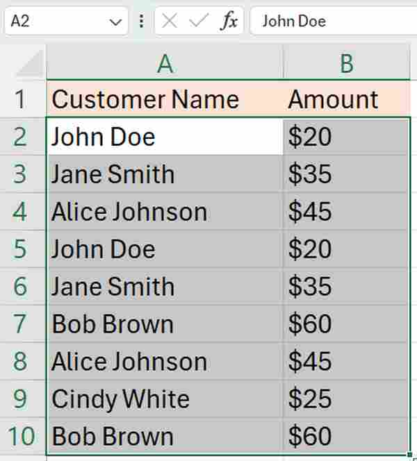
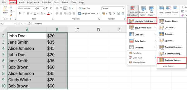
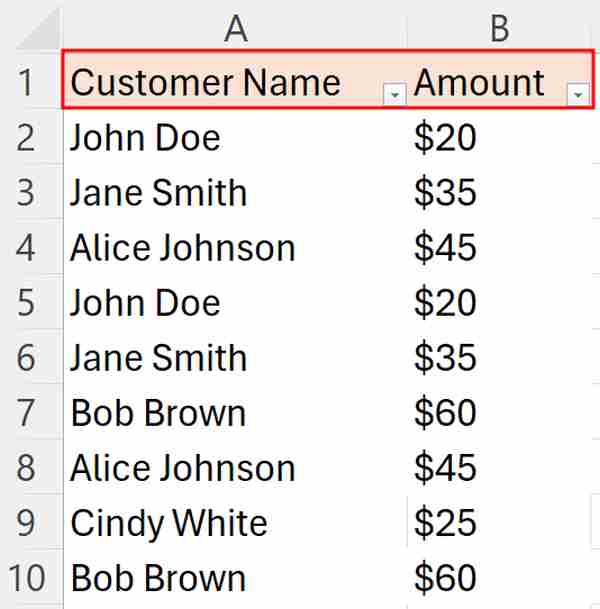
In our example below, click and drag to select the cells containing “Customer Name” and “Amount.” Ensure you include all relevant data you wish to analyze for duplicates. This prepares your dataset for duplicate identification.
2. Apply Conditional Formatting to Identify Duplicates
Click on the ‘Home’ tab at the top of Excel. In the ‘Styles’ group, find and click ‘Conditional Formatting.’ From the dropdown menu, choose ‘Highlight Cells Rules’ and then select ‘Duplicate Values.’
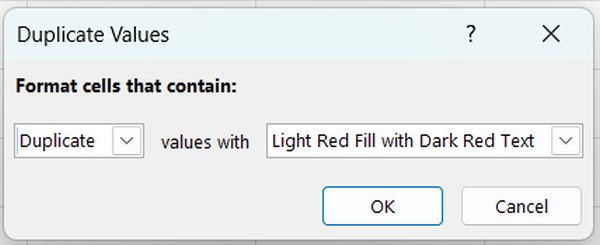
A dialog box will appear, allowing you to choose how duplicates should be highlighted.
3. Choose a Format to Make Duplicates Invisible
In the ‘Duplicate Values’ dialog box, you can choose a formatting style that makes duplicates hard to see.
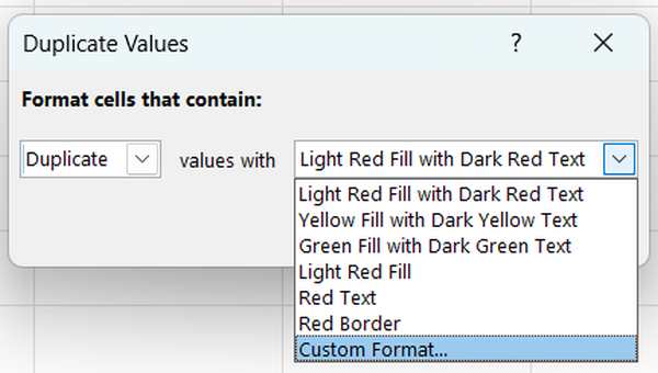
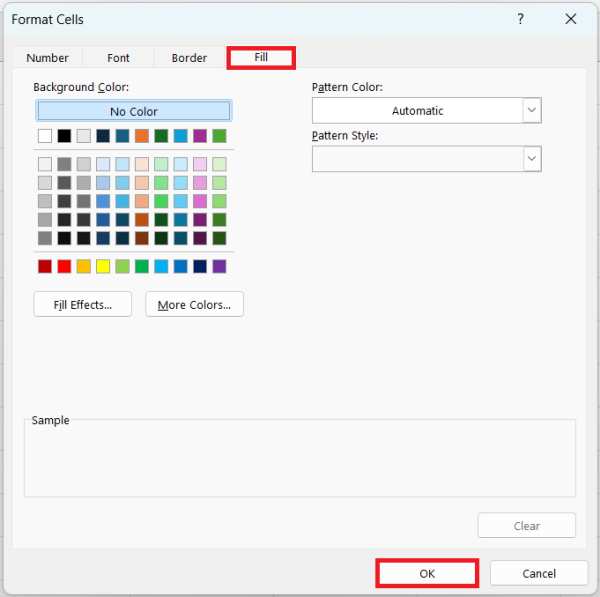
For instance, set the text color to white if your cells are white. Go to ‘Fill’ and choose the color white. This will ‘hide’ the duplicates by making them blend into the background. Click ‘OK’ to apply this formatting across your selected range.
4. Turn On Filtering for Your Data
After highlighting duplicates, activate the filter function to manage visibility. Go to the ‘Data’ tab and click on ‘Filter’.
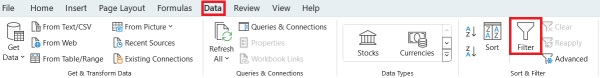
This will add dropdown arrows to the column headers, enabling you to filter the data based on the formatting.
5. Use Filter Options to Hide Duplicated Entries
Click on the dropdown arrow in the header of either the “Customer Name” or “Amount” column. Look for the filter options by color and select ‘No Fill.’
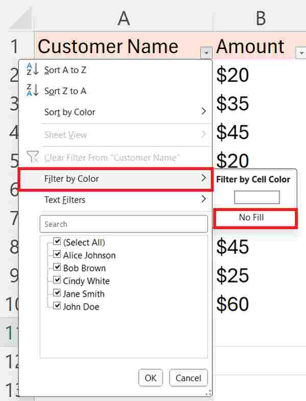
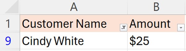
This will effectively hide all rows that contain duplicates, showing only unique data.
Method 2: Using Advanced Filter to Show Only Unique Entries
To hide duplicates in Excel, you can use the Advanced Filter. Here’s how to do it:
1. Select Your Dataset to Filter
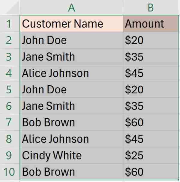
In our example, we have a list of customer names from cells A2 to A10, each paired with their amount in cells B2 to B10. You want to hide the duplicates based on the Customer Name and Amount.
Select the range that includes your headers and all rows of the “Customer Name” and “Amount” columns. This ensures that the filter understands what data to process.
2. Open Advanced Filtering Options
Access the ‘Data’ tab on the ribbon, and click ‘Advanced’ in the ‘Sort & Filter’ section. This action will open the Advanced Filter dialog box where you can specify your filtering criteria.

3. Set the Filter to Show Only Unique Entries
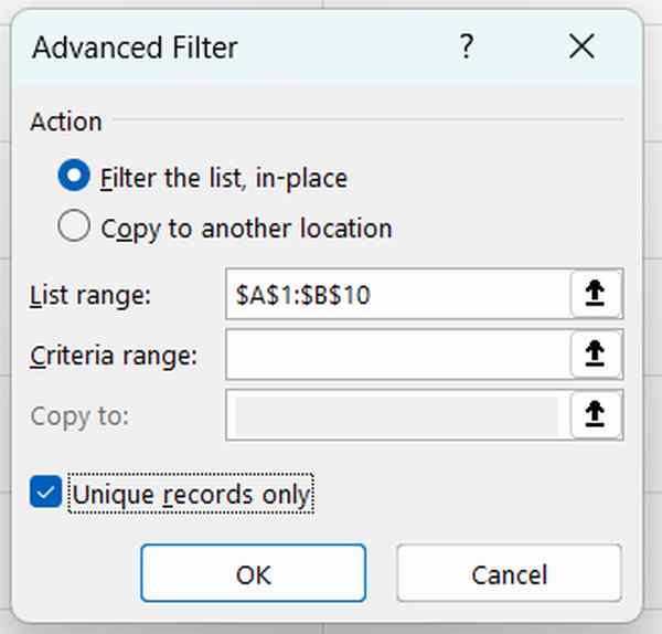
Within the Advanced Filter dialog box, ensure you select ‘Filter the list, in-place.’ Then, mark the checkbox next to ‘Unique records only.’ This tells Excel to modify your displayed data to include only unique items, eliminating any duplicates.
4. Activate the Filter to Remove Duplicates
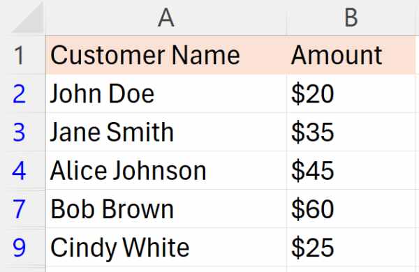
Click ‘OK’ in the Advanced Filter dialog box to apply your settings. The data in your Excel sheet will refresh, now displaying only rows that have unique combinations of names and amounts.
We hope that you now have a better understanding of how to hide duplicates in Excel. If you enjoyed this article, you might also like our article on how to count number of duplicates in Excel or our article on how to remove duplicates in excel but keep one.