How to Split a Cell Horizontally in Excel (Easiest Way in 2025)
In this article, we will learn how to split cells horizontally in Excel by using “Flash Fill”, the “Text to Columns” tool, and the “Fixed Width” option. Simply follow the steps below.
Method 1: How to Split Cells Horizontally in Excel Using “Flash Fill”
Follow the steps below to split cells horizontally in Excel by using “Flash Fill.
1. Create New Columns For Splitting Data
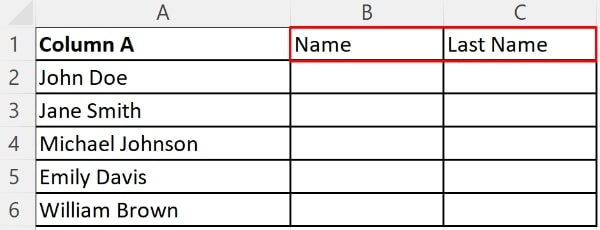
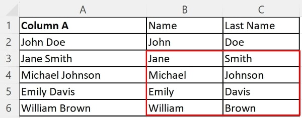
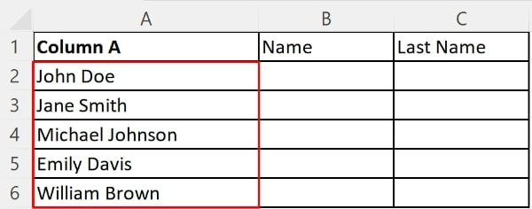
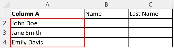
Let’s say we have a list of full names that we want to split into first names and last names. First, ensure that the full names are listed under a single column. Then add two new columns next to the dataset and label them “Name” and “Last Name”.
2. Enter the First Splits Manually
In the first row under “First Name”, type “John”. In the first row under “Last Name”, type “Doe”.

3. Use Flash Fill for the Remaining Rows
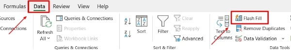
Click the cell in the next row under “First Name”. Then press Ctrl + E or navigate to the Data tab and click on “Flash Fill”. Excel should automatically fill the remaining “First Name” cells.
4. Repeat the Process
Repeat the same process for the “Last Name” column.
Method 2: How to Split Cells Horizontally in Excel Using “Text to Columns”
Follow the steps below to split cells horizontally in Excel using the “Text to Columns” tool.
1. Select the Data to Split
Click and drag to select the cells that contain the data you want to split.
2. Initiate “Text to Columns”
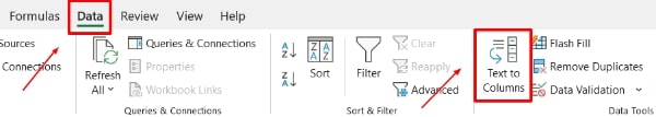
Go to the Data tab on the ribbon at the top of Excel. Then click on “Text to Columns”. This will open the wizard.

3. Set Up the Wizard
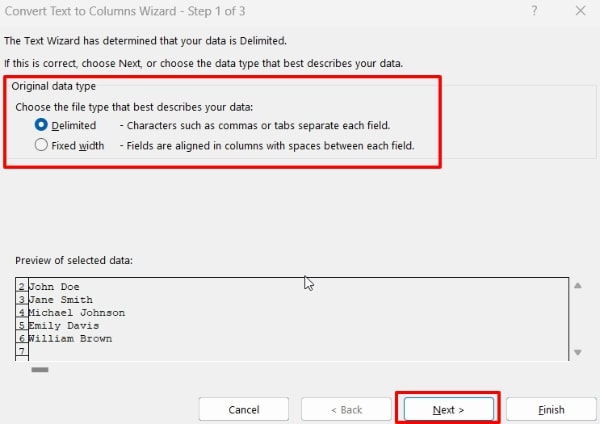
Select “Delimited” in the wizard. This means the data is separated by a delimiter such as a space. Click “Next”.
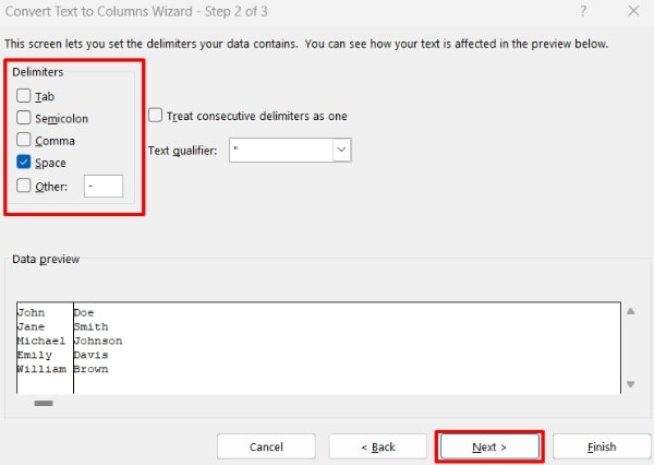
4. Specify Delimiters
Choose “Space” as the delimiter since the first names and the last names are separated by spaces. Click “Next”.
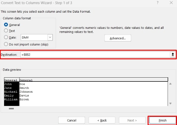
5. Set Up the Destination
Specify where you want the split data to appear. By default, it replaces the original data (Column A), so choose the next column (“Name”) to prevent overwriting. Click “Finish”.
Method 3: How to Split Cells Horizontally in Excel Using “Fixed Width”
Follow the steps below to split cells horizontally in Excel using the “Fixed Width” option.
1. Select the Data to Split
Click and drag to select the cells that contain the data you want to split.
2. Initiate “Text to Columns”
Go to the Data tab on the ribbon at the top of Excel. Then click on “Text to Columns”. This will open the wizard.
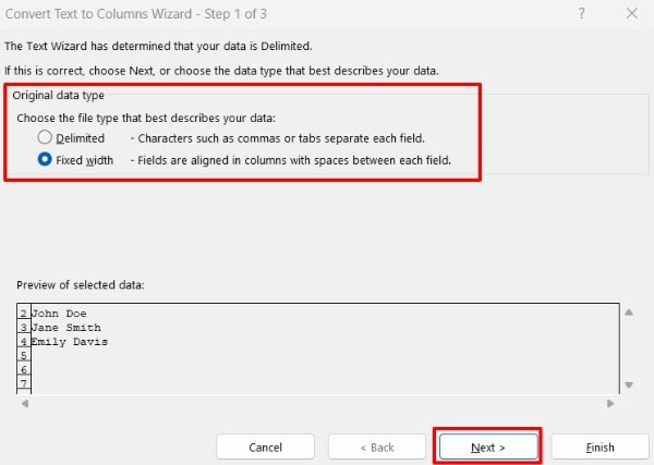
3. Choose the “Fixed Width” Option
Select the “Fixed Width” option then click “Next”.
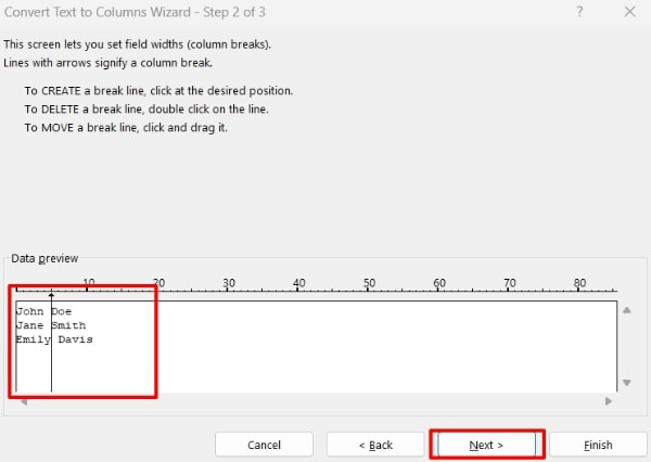
4. Set Break Lines
Click to set break lines in the data preview window at the positions where you want to split the names. Adjust the break line so it falls between the first and last names, typically after the longest first name if the names vary in length. Click “Next”.
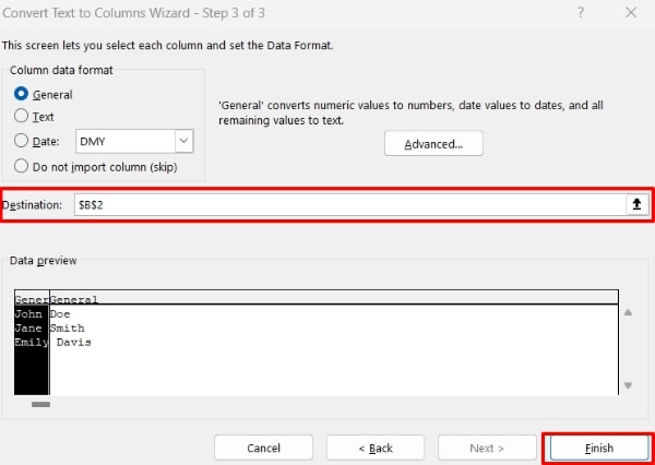
5. Format the Destination
Set the destination for the split data, ideally in columns adjacent to the original data to avoid overwriting. Click “Finish”.
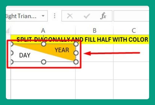
We hope that you now have a better understanding of how to split cells horizontally in Excel. If you enjoyed this article, you might also like our article on how to split email address in excel and how to split cells diagonally in excel.