How to Split Numbers in Excel (Easiest Way in 2025)
In this article, we will learn how to split numbers in Excel by using a formula, the “Flash Fill” function, and the “Text to Columns” tool. Simply follow the steps below.
Method 1: How to Split Numbers in Excel Using a Formula
Follow the steps below to split numbers in Excel by using a formula.
1. Choose an Empty Cell to Display the Extracted Number
First, click on the cell where you want the extracted numbers to appear.
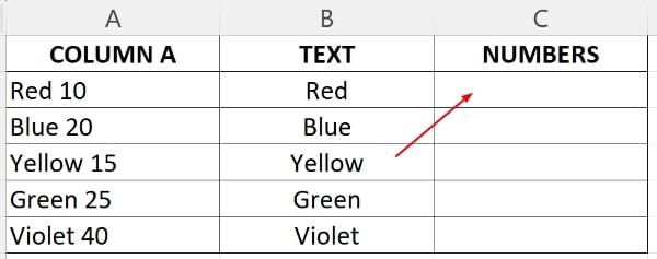
2. Enter the Formula
Enter this formula: “=MID(A1,MIN(FIND({0,1,2,3,4,5,6,7,8,9},A1&”0123456789″)),LEN(A1)+1)“. Replace “A1” with the cell containing your text.

3. Apply the Formula to the Rest of The Cells
Drag the fill handle (a small square at the bottom-right corner of the cell) down to apply the formula to the rest of the cells in the column.
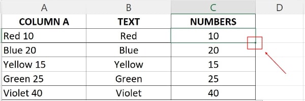
4. Release the Cursor
Release the mouse button to complete the fill action.
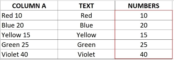
Method 2: How to Split Numbers in Excel Using “Flash Fill”
Follow the steps below to split numbers in Excel using the “Flash Fill” function.
1. Manually Split the First Entry
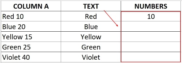
Manually type the desired split for the first entry. In this example, the text is “Red 10” so you should type “10”. Press Enter to confirm the entry.
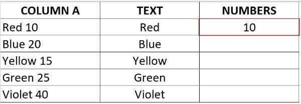
2. Highlight Your Target Range of Cells
Highlight the range of cells where you want the extracted numbers to appear. Include the first cell with the manually entered number.
3. Click on the “Flash Fill” Button
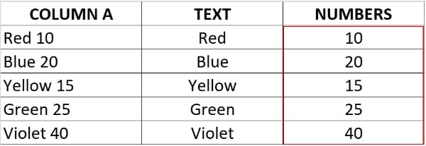
Click on the “Data” tab in the Excel ribbon then click on the “Flash Fill” button. Excel will automatically detect the pattern and fill in the remaining cells with the separated text and numbers.

4. Check Accuracy
Review the filled cells to ensure accuracy. If needed, manually adjust any discrepancies.
Method 3: How to Split Numbers in Excel Using “Text to Columns”
Follow the steps below to split numbers in Excel using the “Text to Columns” tool.
1. Select Your Target Range of Cells
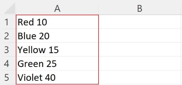
Select the column containing the text and numbers you want to split.
2. Select the “Text to Columns” Button
Click on the “Data” tab in the Excel ribbon then click on the “Text to Columns” button.

3. Choose “Delimited”
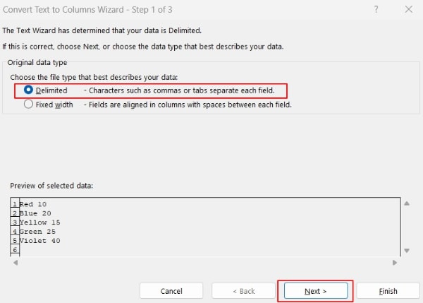
The “Convert Text to Columns Wizard” window will open. Choose “Delimited” and click “Next.”
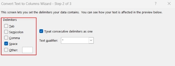
4. Select the Delimiter
Select the delimiter that separates your text and numbers (e.g., space, comma, etc.). In this sample dataset, the delimiter is Space.
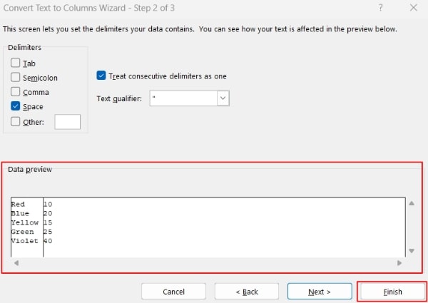
5. Review the Data Preview
If your text and numbers have a consistent format, review the data preview and adjust settings as needed. Click “Finish” when satisfied.
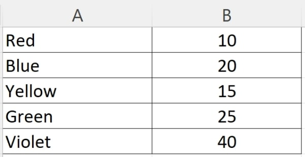
6. Check Accuracy
Excel will split the text and numbers into separate columns. Review the filled cells to ensure accuracy.
We hope that you now have a better understanding of how to split text and numbers in Excel. If you enjoyed this article, you might also like our article on how to freeze the second row in Excel and how to split addresses in Excel.

