List Box in Excel: The Ultimate Guide for 2025
In this article, we will show you how to create a list box in Excel. Simply follow the steps below.
How to Create a List Box in Excel
Follow the steps below on how to create a list box in Excel.
1. Prepare Data for List Box
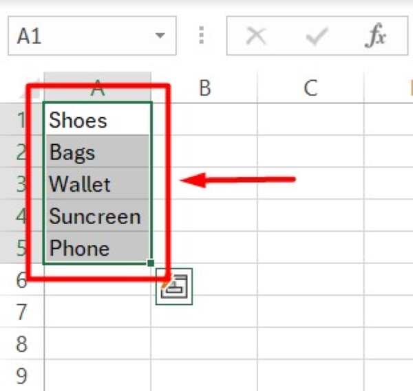
Ensure you have the data ready that you want to use for the list box. Enter your list items in a single column, one item per cell. For example, enter “Shoes” in cell A1, “Bags” in cell A2, and so on.
2. Select Cell for List Box Location
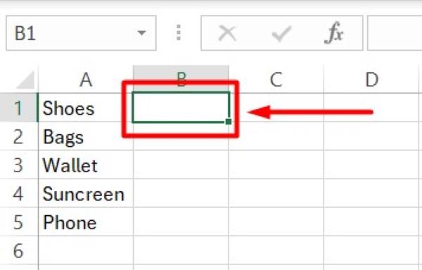
Click on the cell where you want the list box to appear. This is where users will click to see the dropdown menu. For instance, you might select cell B1 if you want the list box there.
3. Navigate to Data Validation Tool
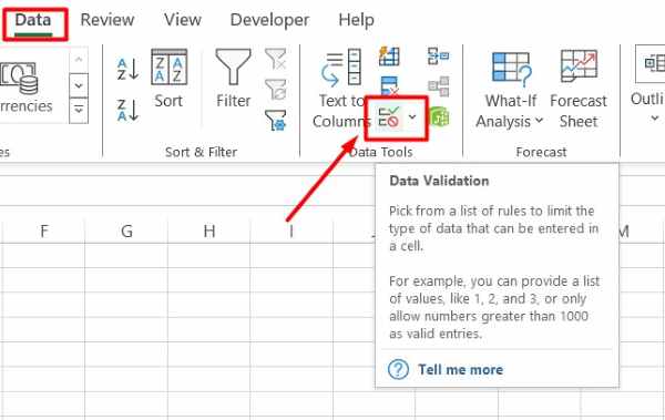
Go to the “Data” tab on the ribbon at the top of Excel. In the “Data Tools” group, click “Data Validation.” A dialog box will open, allowing you to set up the list box.
4. Set Data Validation to List Option
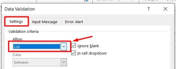
In the Data Validation dialog box, go to the “Settings” tab. Under the “Allow” dropdown menu, choose “List.” This option specifies that you want to create a list from which users can select an item.
5. Define List Items or Range
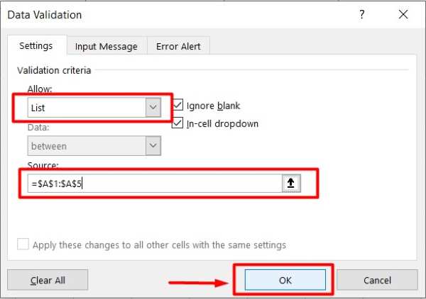
Click in the “Source” box. Next, select the range of cells containing your list items. Click and drag to highlight your list, or manually enter the range (e.g., A1:A5). You can also type the items directly into the box, separated by commas (e.g., Item1, Item2, Item3). Click “OK” to close the Data Validation dialog box.
6. Confirm and Create List Box
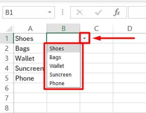
Now, click the cell you selected for the list box (e.g., B1). A dropdown arrow will appear, indicating the list box is ready. Click the arrow to see and select items from your list.
We hope you now have a better understanding of how to create a list box in Excel. If you enjoy this article, you might also like our article on how to put checkbox in Excel or our article on ways to create Excel multi-select listbox.

