Return All Rows That Match Criteria in Excel (2025 Guide)
In this article, we will show you how to return all rows that match criteria in Excel. Simply follow the steps below.

Find Rows That Match Criteria in Excel
Follow the steps below to return the rows that match criteria in Excel.
1. Locate the Predefined Criteria Range
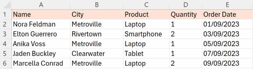
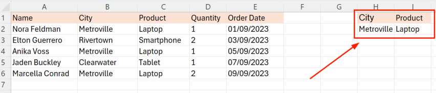
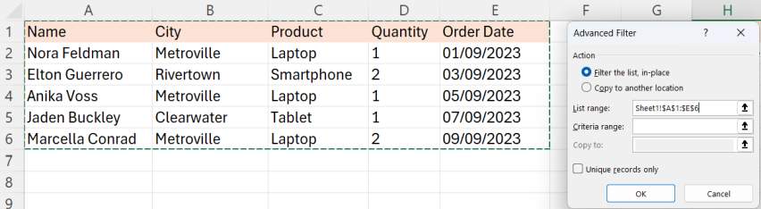
Find the area on your worksheet where the criteria range is already set up. In our example, we have a list of customer orders from rows 1 to 5, detailing names, cities, products, quantities, and order dates.
We want to filter and display only those entries where the city is “Metroville” and the product is a “Laptop.”
2. Prepare Your Criteria Range
Set up a section on your worksheet specifically for your filter conditions, known as the ‘Criteria Range’. Locate this area separate from your main data, often at the top or on a separate part of the worksheet.
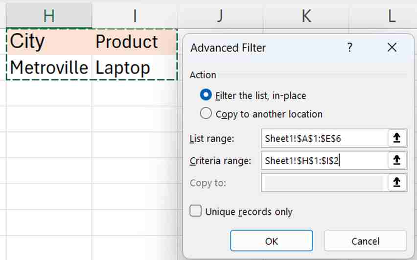
For example, we will label “City” as the header in cell H1, and “Product” as the header in cell I1. Directly below these headers, we will specify the filter conditions by placing “Metroville” in cell H2 under the “City” header and “Laptop” in cell I2 under the “Product” header.
3. Access the Advanced Filter Function in Excel
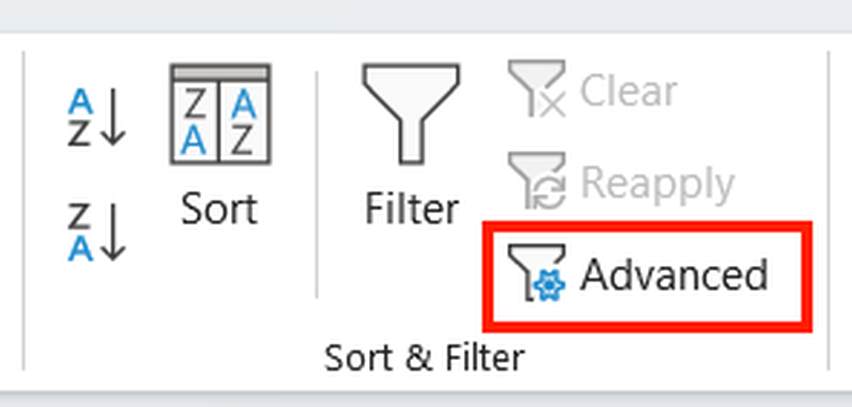
Navigate to the ‘Data’ tab on the menu bar at the top of your screen and find the ‘Sort & Filter’ group.
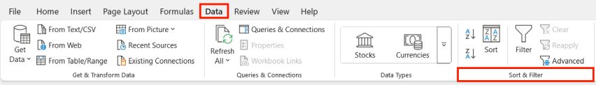
Here, click on ‘Advanced’ to open the Advanced Filter dialog box. This tool allows you to set more specific filter rules than the standard filter options.
4. Set Up and Apply the Advanced Filter to Your Data
Once the Advanced Filter dialog box is open, select the option ‘Filter the list, in-place’ to filter your data directly on the current worksheet.
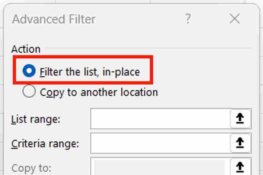
Next, you need to specify two important areas in your Excel sheet: The List Range and Critera Range.
The List Range is the area that contains all your data that you want to filter. For our example, we will select the cells from A1 to E6. This includes the headers and all the rows of customer order data.
The Criteria Range is where you have specified the conditions for filtering. In our example, we will select the range H1:I2.
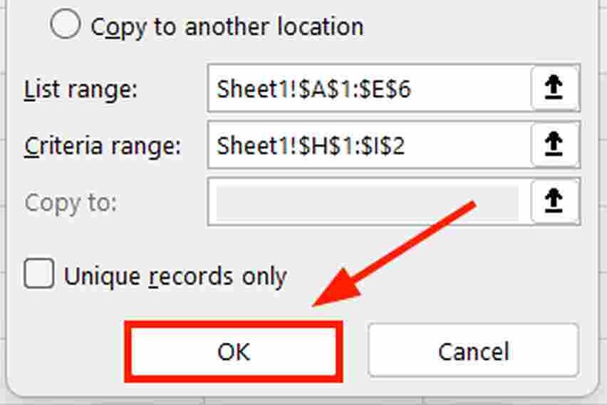
After selecting both ranges, click ‘OK’ in the Advanced Filter dialog box to execute the filter.
5. Review the Results to Ensure Correct Data Filtering
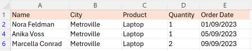
Examine your worksheet to confirm that it now only shows the rows matching your criteria: entries from Metroville involving laptops. If you see only these rows, your filter has been applied correctly.
We hope that you now have a better understanding of how to return all the rows that match your criteria in Excel. If you enjoyed this article, you might also like our articles on how to return all values that match criteria in Excel and on applying the index match formula with multiple criteria in Excel.