How to Unfreeze Panes in Excel (Easiest Way in 2025)
In this article, we will show you how to unfreeze panes in Excel. Simply follow the steps below.
Unfreeze Panes in Excel
To unfreeze panes in Excel, you can consider three common aspects: rows, columns, and cells. We’ll show you how to unfreeze each one in the following sections.
How to Unfreeze Rows in Excel
Follow the steps below on how to unfreeze ROWS in Excel.
1. Identify the Frozen Rows in your Excel Sheet
Locate the rows that are currently frozen in your Excel sheet. These rows remain visible when you scroll through the rest of the data.
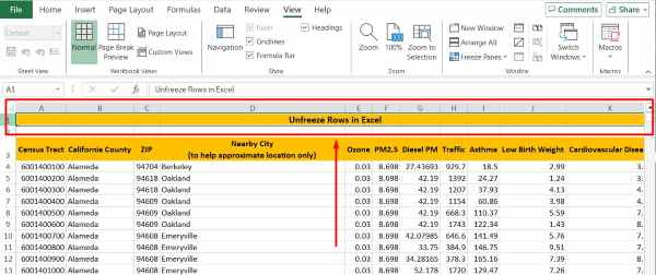
2. Select “Freeze Panes” from the Toolbar
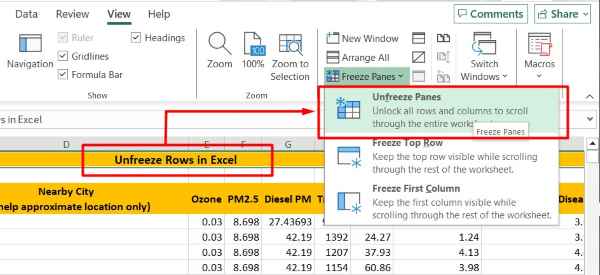
Find the “View” tab at the top of the Excel window and click on it to access the view-related options. In the “View” tab, locate and click on “Freeze Panes.” This will reveal a dropdown menu.

3. Choose “Unfreeze Panes” from the Dropdown Menu
From the dropdown menu that appears after clicking “Freeze Panes,” select the “Unfreeze Panes” option. This action will remove the frozen rows from your spreadsheet.
How to Unfreeze Columns in Excel
Follow the steps below on how to unfreeze COLUMNS in Excel.
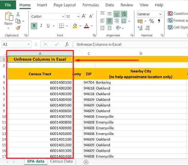
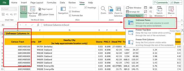
1. Identify the frozen columns.
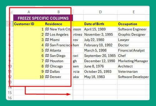
Locate the columns that are currently frozen in your Excel sheet. These columns remain visible when you scroll through the rest of the data.
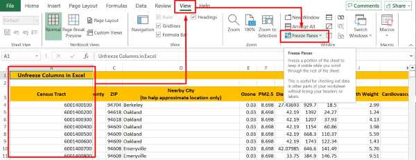
2. Access “Freeze Panes” from the toolbar.
Find the “View” tab at the top of the Excel window and click on it to access the view-related options. In the “View” tab, locate and click on “Freeze Panes.” This will reveal a dropdown menu.
3. Select “Unfreeze Panes” from the dropdown menu.
From the dropdown menu that appears after clicking “Freeze Panes,” select the “Unfreeze Panes” option. This action will remove the frozen columns from your spreadsheet.
How to Unfreeze Cells in Excel
Follow the steps below on how to unfreeze CELLS in Excel.
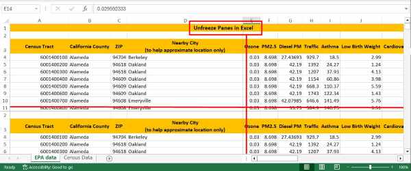
1. Identify the frozen cells or panes.
Locate the cells that are currently frozen in your Excel sheet. These cells remain fixed in place when you scroll through the rest of the data.
2. Click on the “View” tab to Access Options
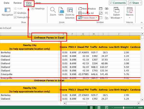
Find the “View” tab at the top of the Excel window and click on it to access the view-related options. Select “Freeze Panes” from the toolbar. In the “View” tab, locate and click on “Freeze Panes.” This will reveal a dropdown menu.
3. Choose “Unfreeze Panes” from the dropdown menu.
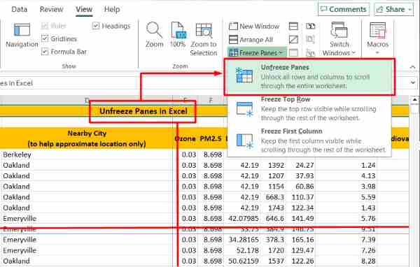
From the dropdown menu that appears after clicking “Freeze Panes,” select the “Unfreeze Panes” option. This action will remove the frozen cells from your spreadsheet.
We hope you now better understand how to unfreeze panes in Excel. If you enjoyed this article, you might also like our article on ways to merge cells in Excel and keep all text or our article on how to freeze title row in Excel.

