IMPORTRANGE in Excel (How to Use it in 2024)

In this article we will explore Excel’s IMPORTRANGE function with clear examples and visual guides for streamlined data management.

How to Import Range in Excel

While Excel lacks an equivalent of the IMPORTRANGE function in Google Sheets, you can get similar results by using Excel’s features. Simply follow the steps below.

1. Select the Destination Cell

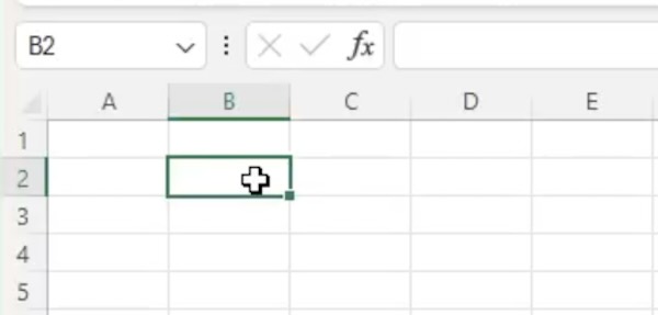
Click on the cell where you want to import the data in the destination spreadsheet. In the example below, we select cell B2.

2. Enter the Formula

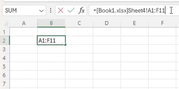
Enter the formula in the selected cell:

=[Source.xlsx]Sheet1!A1:J10

Replace “Source.xlsx” with the name of the source Excel file, “Sheet1” with the name of the source worksheet, and “A1:J10” with the range you want to import.

3. Press Enter

Press Enter after entering the formula. The data from the specified cell in the source spreadsheet will be imported into the selected cell in the destination spreadsheet.

We hope you now have a better understanding of the IMPORTRANGE equivalent in Excel. If you enjoyed this article, you might also like our article on how to import Excel into Powerpoint or our article on how to import data from a website to Excel.