How to Find Duplicate Values in Excel Using VLOOKUP (2024)

In this article we will show you how to find duplicate values across two columns in Excel using VLOOKUP. Simply follow the steps below.

How to Find Duplicate Values in Two Columns in Excel Using VLOOKUP

To use VLOOKUP in finding duplicate values in Excel, simply follow the steps below.

1. Prepare Your Excel Worksheet

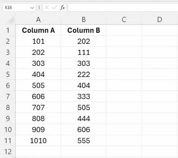
Ensure your Excel worksheet has the two columns you want to compare. Label each column clearly to avoid confusion. For our example, imagine we have two columns labeled ‘Column A’ and ‘Column B’.

2. Create a Helper Column

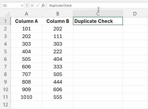
Next to Column B, add a new column labeled ‘Duplicate Check’. This column will display the results of the VLOOKUP formula, helping you identify duplicates between Column A and Column B.

3. Enter the VLOOKUP Formula

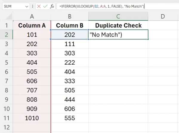
In the first cell of the ‘Duplicate Check’ column, enter the VLOOKUP formula:

=IFERROR(VLOOKUP(B2, A:A, 1, FALSE), "No Match")

This formula checks each value in Column B against all values in Column A. If a duplicate is found, it shows the value; if not, it shows “No Match”.

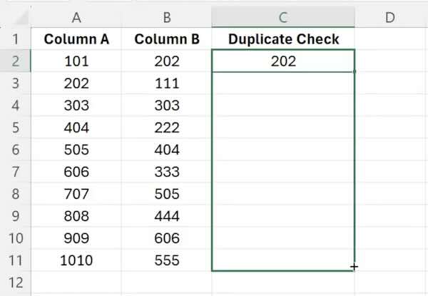
4. Copy the Formula Down

Drag the fill handle (small square at the bottom-right corner of the cell) down through the column to apply the formula to all other cells in the ‘Duplicate Check’ column. This will extend the duplicate search to all listed entries in Column B.

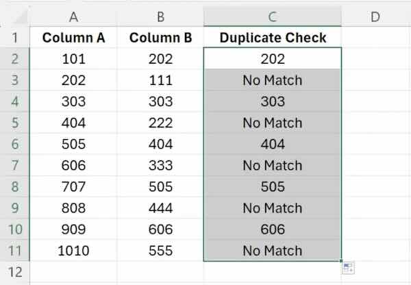
5. Analyze the Results

Review the ‘Duplicate Check’ column. Values that appear in both Column A and Column B are listed by their names, indicating they are duplicates. Values unique to Column B are labeled as “No Match”.

We hope you now have a better understanding of how to find duplicate values in Excel using VLOOKUP. If you enjoyed this article, you might also like our article on how to import data from another workbook in Excel or our article on how to duplicate an Excel file.