Compare Two Lists for Matches in Excel (Easiest Way in 2024)

In this article, we will show you how to compare two lists for matches in Excel. Simply follow the steps below.

How to Compare Two Lists in Excel for Matches

Two lists can be compared in Excel for matches using four effective methods: the ‘Conditional Formatting’ technique, the ‘IF’ function, the ‘Go To Special’ Technique, and the ‘VLOOKUP’ function. We will cover how to use each method in the following sections.

Method 1: Compare Lists Using Conditional Formatting

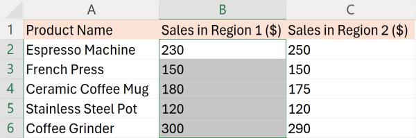
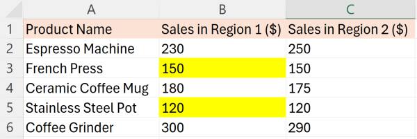
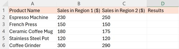
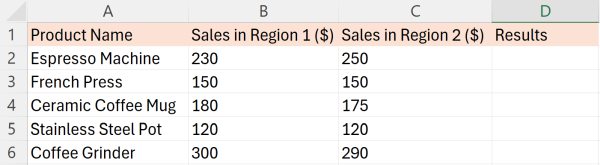
To compare lists for matches in Excel, we will work with a dataset containing product names in Column A, sales in Region 1 in Column A, and sales in Region 2 in Column B. Follow the steps below:

1. Select Region 1 Sales Data

Click on the first cell under the “Sales in Region 1 ($)” column at B2 and drag down to select all the sales data in that column. Ensure that your selection includes all rows containing sales figures.

2. Access Conditional Formatting Tools

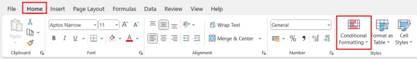
Navigate to the ‘Home’ tab on the Excel ribbon. Locate the ‘Styles’ group and click on ‘Conditional Formatting’ to open its dropdown menu.

3. Create a New Rule to Highlight Matching Sales

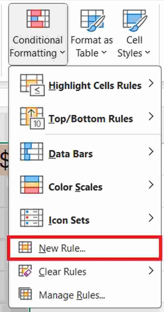
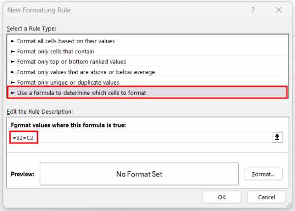
Click on ‘New Rule’ within the Conditional Formatting options. 

Choose ‘Use a formula to determine which cells to format.’ Enter the formula =B2=C2 in the formula box to compare the sales figures between Region 1 and Region 2 for each row. 

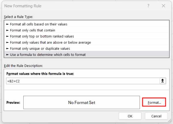
4. Configure the Highlighting Format

Click the ‘Format…’ button within the new rule configuration. 

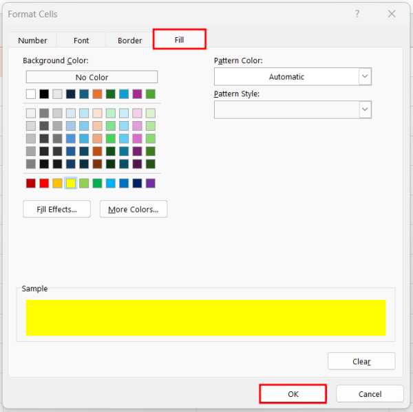
In the ‘Format Cells’ dialog, select the ‘Fill’ tab. Choose a background color, such as yellow, to apply to cells where the sales figures match. This visual indication will make it easy to spot matching figures. After selecting the color, click ‘OK’ to close the ‘Format Cells’ dialog, then click ‘OK’ again to apply the rule.

5. Review the Highlighted Matches

Once the rule is applied, you’ll see that cells in column B that have matching figures in column C are highlighted in yellow. This indicates where the sales amounts for Region 1 correspond exactly to those for Region 2, allowing you to quickly identify matched sales figures between the two regions.

Method 2: Identify Matches Using IF in a Helper Column

Below, we outline the steps on how to compare two lists in Excel for matches using the IF function in a helper column.

1. Insert a Helper Column for Comparison Results

In our example, we have a list of sales in Region 1 from cells B2 to B6 and sales in Region 2 from cells C2 to C6. 

Add a new column immediately to the right of your “Sales in Region 2 ($)” column. This column will be used to display the results of the comparison. In our case, it will be column D.

2. Input Comparison Formula in the New Column

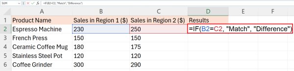
In the first cell of your newly added column (cell D2), enter the formula `=IF(B2=C2, “Match”, “Difference”)`. This formula checks if the sales figures in columns B and C are equal. If they are, “Match” will be displayed; otherwise, “Difference”.

3. Extend the Comparison Formula Down the Column

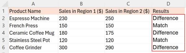
Click on the cell where you entered the formula, then drag the fill handle (the small square at the bottom-right corner of the cell) down through the column to copy the formula to other rows. This will apply the comparison to all listed items.

Method 3: Use Go To Special to Find Differences in Pasted Data

Follow the steps below to compare the sales of products between two regions using the ‘Go To Special’ technique.

1. Select All Cells Containing Sales Data

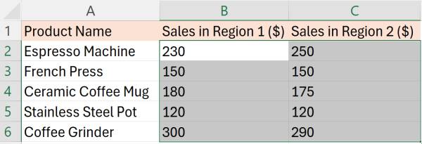
Select both columns containing sales data for Regions 1 and 2. 

2. Open Go To Special for Sales Comparison

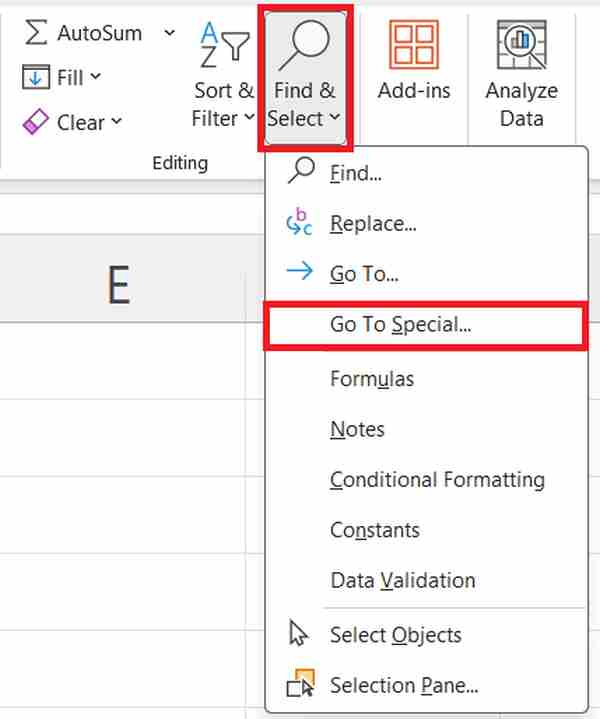
Navigate to the ‘Home’ tab, click ‘Find & Select’, then choose ‘Go To Special’. 

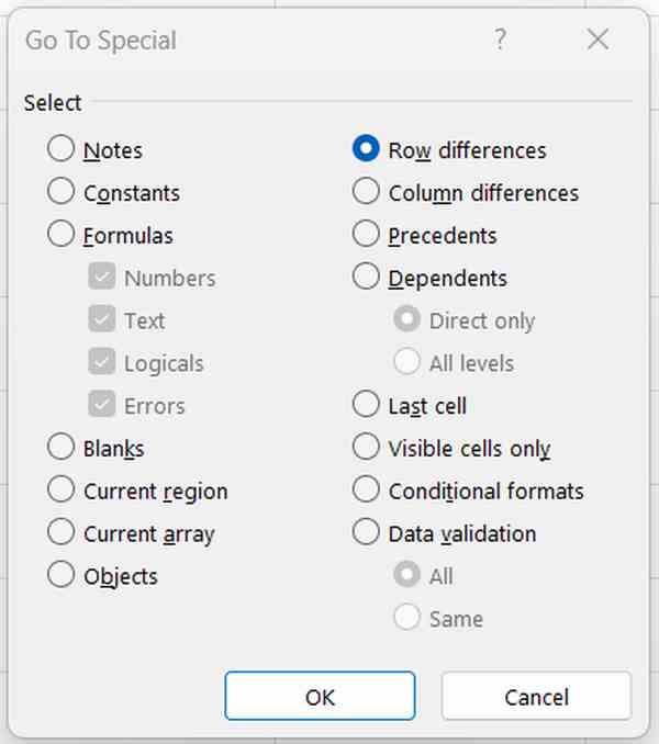
In the dialog box that appears, select ‘Row differences’. This option will highlight cells in the “Sales in Region 2 ($)” column where the contents differ from those in the “Sales in Region 1 ($)” column.

3. Apply Color Fill to Highlight Differences

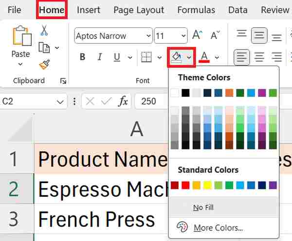
Once Excel highlights the differences, you can easily apply a color fill to make these differences stand out visually. Go to the ‘Home’ tab, click on the ‘Fill Color’ icon in the Font group, and choose a color such as yellow. This will fill the highlighted cells in Column C with yellow, making it very clear where discrepancies between the sales data in Region 1 and Region 2 occur.

Method 4: VLOOKUP to Match Sales Data

In order to compare two lists for matches in Excel, simply follow the steps below. 

1. Prepare a Column for VLOOKUP Results

In our example, we have a list of sales in Region 1 in Column B and sales in Region 2 in Column C.

Create a new column to the right of the “Sales in Region 2 ($)” column for displaying VLOOKUP results. This should ideally be the next empty column after your sales data. In our case, this will be column D.

2. Implement the VLOOKUP Formula for Sales Comparison

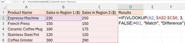
In the first cell of this new column (cell D2), type:

=IF(VLOOKUP(A2, $A$2:$C$6, 3, FALSE)=B2, “Match”, “Difference”) 

Where:

A2: The product name you are searching for.

$A$2:$C$6: The data range containing the product names and their sales figures for both Region 1 (Column B) and Region 2 (Column C). The dollar signs fix the range so it doesn’t change as the formula is copied down.

3: The column index number indicating that the sales figures from Region 2 (the third column in the defined range) are to be returned.

FALSE: Specifies that VLOOKUP should find an exact match for the product name in A2.

=B2: Compares the result from VLOOKUP (Region 2 sales) with the sales figure in Region 1 (B2).

IF(…, “Match”, “Difference”): Outputs “Match” if the sales figures are equal; otherwise, outputs “Difference”.

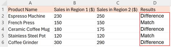
3. Apply the VLOOKUP Formula to All Products

Copy the formula by dragging the fill handle of the cell downwards to fill the formula across all products listed. This step ensures each product is checked for matching sales figures across the regions.

We hope that you now have a better understanding of how to compare two lists for matches in Excel. If you enjoyed this article, you might also like our article on how to compare two columns in Excel and return value from another column or our article on how to compare two columns in Excel for matches.