Formula to Compare Two Columns and Return a Value in Excel
In this article, we will explore how to compare two columns and return a value in Excel. Simply follow the steps below.
Compare Two Columns in Excel and Return Common Values
“Two columns can be compared to return common values in Excel using three effective methods: the “EQUALS” operator, the “IF Condition”, and the “EXACT” function. We will discuss how to use each method in the following sections.
Method 1: Compare Using EQUALS Operator for Exact Matches
Below, we outline the steps on how to compare two columns in Excel and return the value from another column.
1. Insert EQUALS Formula to Check for Matches
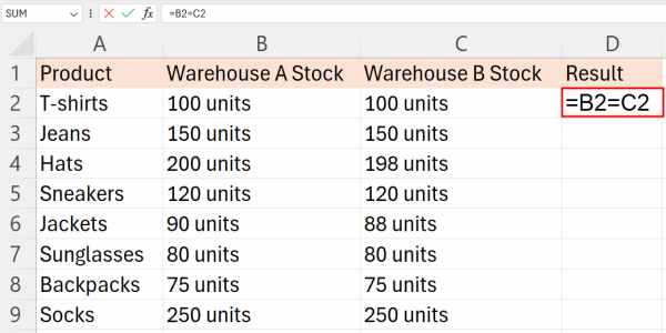
In our example, we have a table that compares product stock levels from two different warehouse locations for a list of products.
In a column next to your data, enter the formula ‘=B2=C2’ in the first cell below the column header (cell D2). This formula checks whether the stock levels in corresponding rows of Warehouse A and Warehouse B are exactly the same.
2. Copy the Formula Down
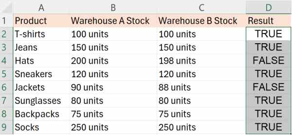
Select the cell where you just typed the formula. Drag the fill handle (the small square at the bottom-right corner of the cell) down to apply this formula to all rows below. This action will fill each cell in the column with TRUE if the quantities match exactly, and FALSE if they do not.
Method 2: Use IF Condition to Label Matching and Non-matching Entries
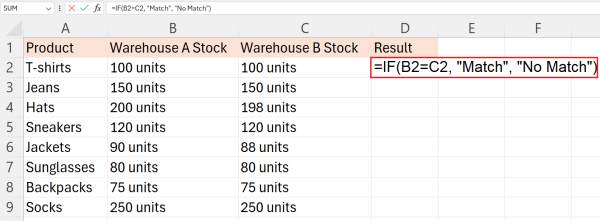
To compare two columns in Excel and return common values, we will work with a dataset containing product names in Column A, warehouse A stock in Column B, and warehouse B stock in Column C. Follow the steps below:
1. Apply the IF Function to Indicate the Match Status
In another new column (Column D), enter the formula `=IF(B2=C2, “Match”, “No Match”)‘ in the first cell (cell D2). This IF function checks each row to determine if the stock levels in Warehouses A and B match.
2 Copy the IF Function Down
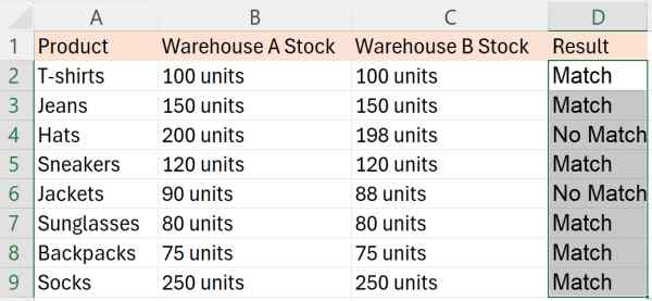
Drag the fill handle down the column to extend the formula to all necessary rows. If the stocks in A in B are equal, it returns “Match”; if they differ, it returns “No Match”.
Method 3: Use EXACT Function for Case-Sensitive Comparisons
Follow the steps below to compare stock levels of products between two warehouses using the EXACT function.
1. Compare Columns with EXACT for Precise Matches
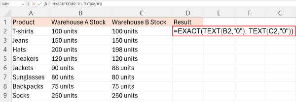
In the column next to Warehouse B’s stock, enter the formula `=EXACT(TEXT(B2,”0″), TEXT(C2,”0″))‘ in the first row that contains data (cell D2). The EXACT function performs a case-sensitive comparison of the stock figures, considering them as text.
2. Copy the EXACT Function Down
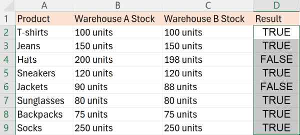
Select the cell where you entered the EXACT formula and drag the fill handle down to extend this formula to the rest of the rows. This action applies the case-sensitive comparison to all listed products, showing TRUE for exact matches and FALSE for any discrepancies.
We hope that you now have a better understanding of the formula to compare two columns and return a value in Excel. If you enjoyed this article, you might also like our article on how to use conditional formatting to compare two columns in Excel or our article on how to compare two lists in Excel for matches.

