Excel Conditional Formatting to Compare Columns (2025 Update)
In this article, we will show you how to use conditional formatting to compare two Excel columns. Simply follow the steps below.
Conditional Formatting in Excel to Compare Two Columns
To compare two columns using Excel conditional formatting greater than, simply follow the steps below.
1. Select the Data Range
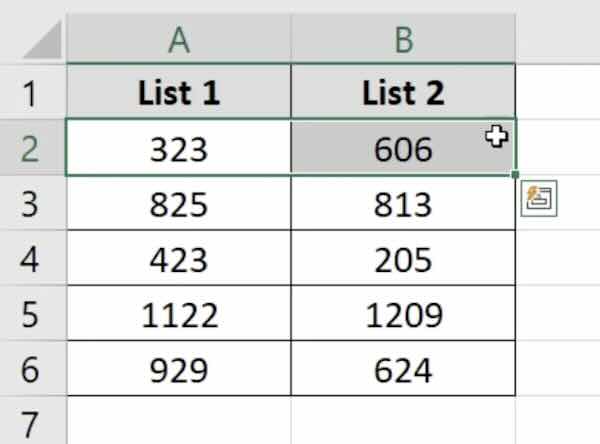
Highlight the cells in the first column that you want to compare. For example, if you want to compare column A and column B, select the data range in column A first.
2. Access Conditional Formatting
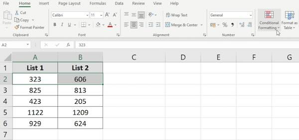
Go to the “Home” tab on the ribbon. In the “Styles” group, click on “Conditional Formatting.” This will open a dropdown menu with various formatting options.
3. Create a New Rule
From the “Conditional Formatting” dropdown menu, choose “New Rule.” This will open the “New Formatting Rule” dialog box.
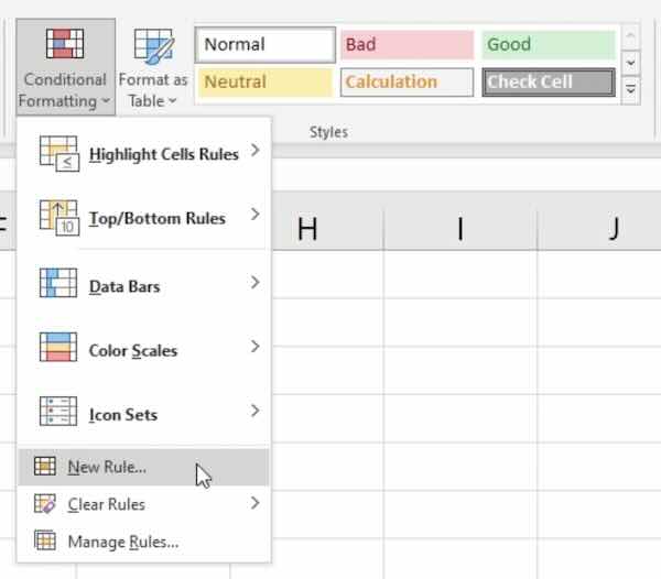
4. Use a Formula to Determine Which Cells to Format
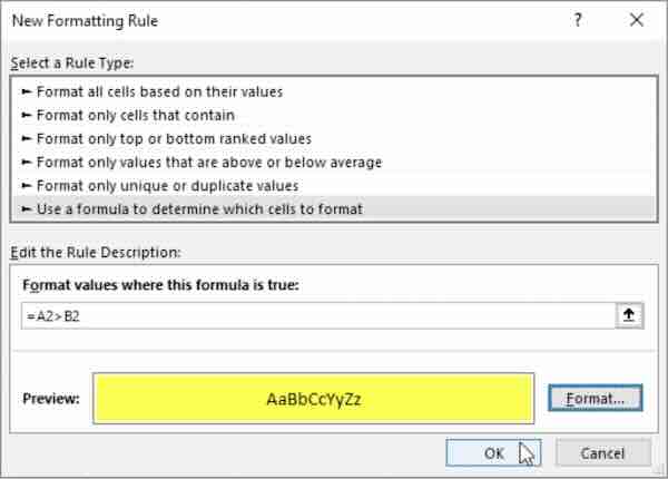
In the “New Formatting Rule” dialog box, select “Use a formula to determine which cells to format.” This option lets you apply custom formulas for conditional formatting.
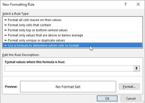
5. Enter the Comparison Formula
In the formula field, enter the formula to compare the two columns. For example, to highlight cells in column A that are greater than those in column B, type =A1>B1.
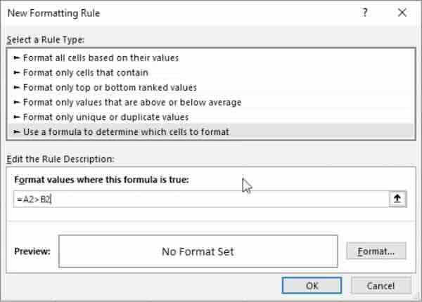
6. Choose a Formatting Style
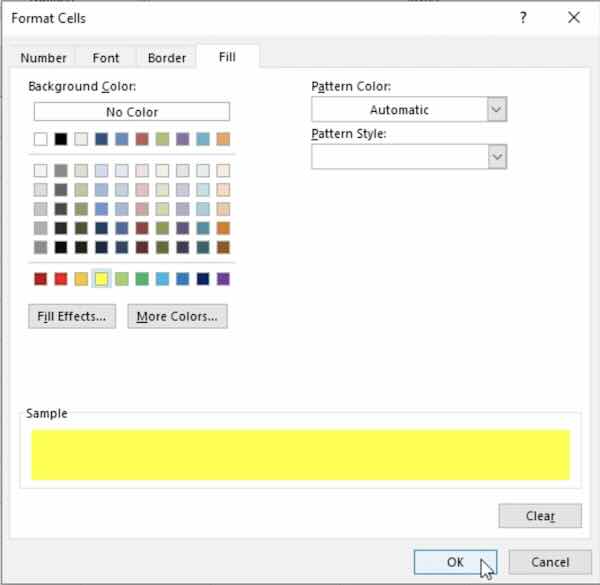
Click the “Format” button to choose how you want the cells to be highlighted if the condition is met. You can choose different colors, fonts, or borders.
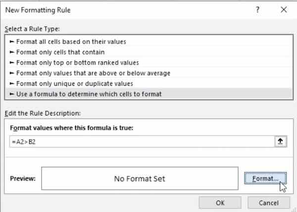
7. Apply the Formatting
After selecting your formatting style, click “OK” in the “Format Cells” dialog box. Then, click “OK” again in the “New Formatting Rule” dialog box. The cells in column A that are greater than those in column B will be highlighted.
8. Copy the Formatting Rule
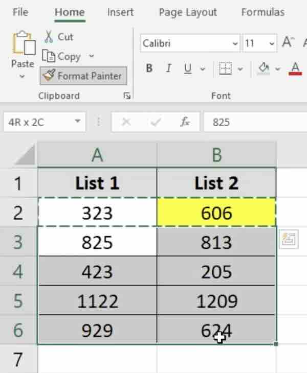
If you want to apply the same rule to other cells, use the Format Painter tool. Select the formatted cells, click on the Format Painter, and then highlight the new range of cells.
We hope you now have a better understanding of how to use conditional formatting in Excel to compare two columns. If you enjoyed this article, you might also like our article on how to compare two columns in Excel to find differences or our article on how to compare two columns in Excel and return common values.

