Conditional Formatting Duplicates in Excel (Easiest Way in 2024)

In this article, we will show you how to use conditional formatting to identify duplicates in Excel. Simply follow the steps below.

Excel’s Conditional Formatting for Duplicates

To spot duplicates using conditional formatting in Excel, simply follow the steps below.

1. Select the Data You Want to Find Duplicates

Select the range of cells where you want to find duplicates. Click on the first cell and drag to the last cell in the range.

2. Open Conditional Formatting

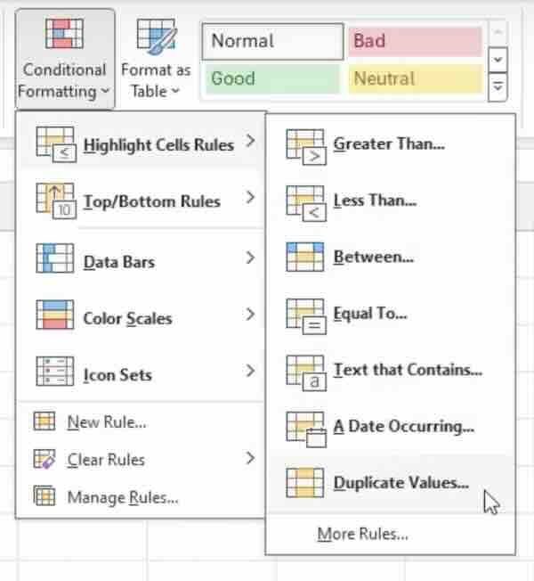
Go to the ‘Home’ tab on the Excel ribbon. Click on ‘Conditional Formatting’ in the ‘Styles’ group.

3. Choose Highlight Rules

From the conditional formatting menu, hover over ‘Highlight Cells Rules.’ A side menu will appear. Select ‘Duplicate Values’ from this list.

4. Set Formatting Options

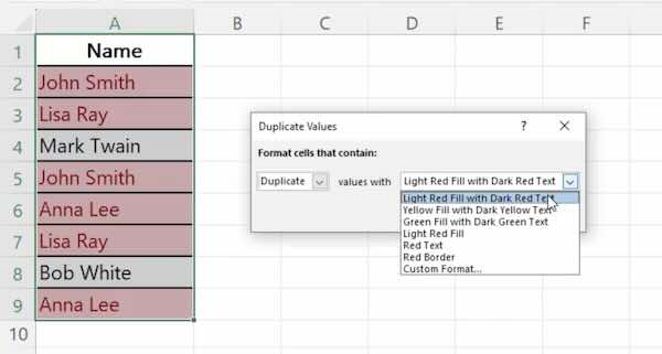
In the ‘Duplicate Values’ dialog box, choose a format for highlighting duplicates. You can select from predefined styles or customize your own. Click ‘OK’ when done.

We hope you now have a better understanding of how to use conditional formatting to identify duplicates in Excel. If you enjoyed this article, you might also like our article on how to group duplicates in Excel or our article on how to generate random numbers in Excel without duplicates.