How to Filter Merged Cells in Excel (Easiest Way in 2025)
In this article, we will show you how to filter merged cells in Excel. Simply follow the steps below.
How to Filter in Excel with Merged Cells
Follow the process below to easily filter merged cells in Excel.
1. Select the Range of Merged Cells
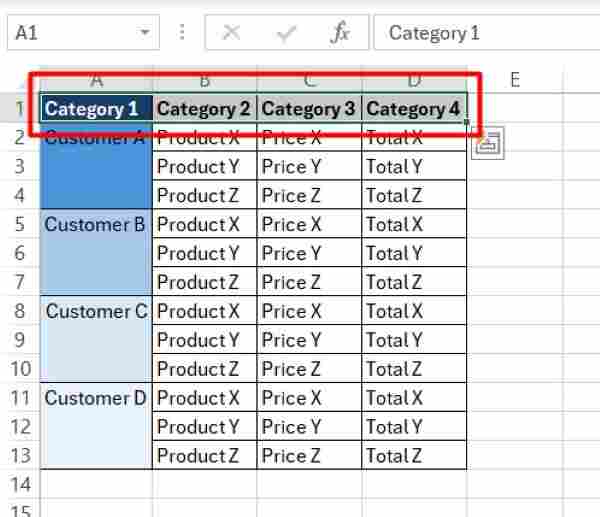
Click and drag to select the range of merged cells you want to filter. Ensure your selection covers all the merged cells you want to work with.
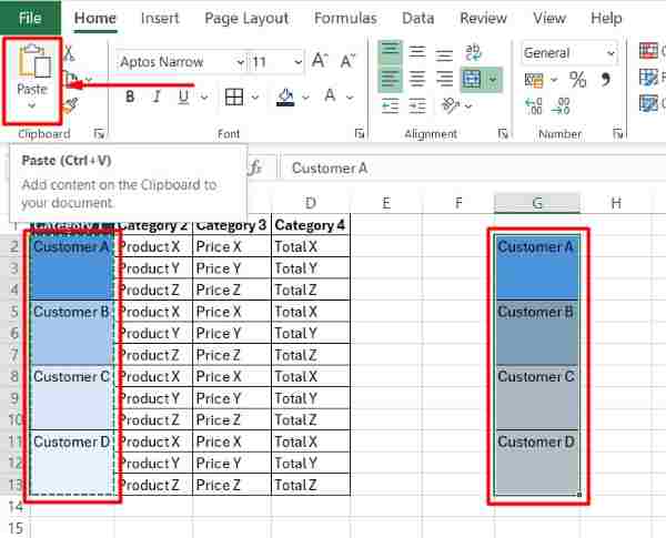
After that, “copy” and “paste” the merged cells into different cells to reserve the format for later.
2. Unmerge the Selected Cells
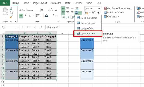
Before applying filters, unmerge the selected cells. Navigate to the “Home” tab, find the “Merge & Center” button in the Alignment group, and select “Unmerge Cells.”
3. Replicate the Merged Cell Content
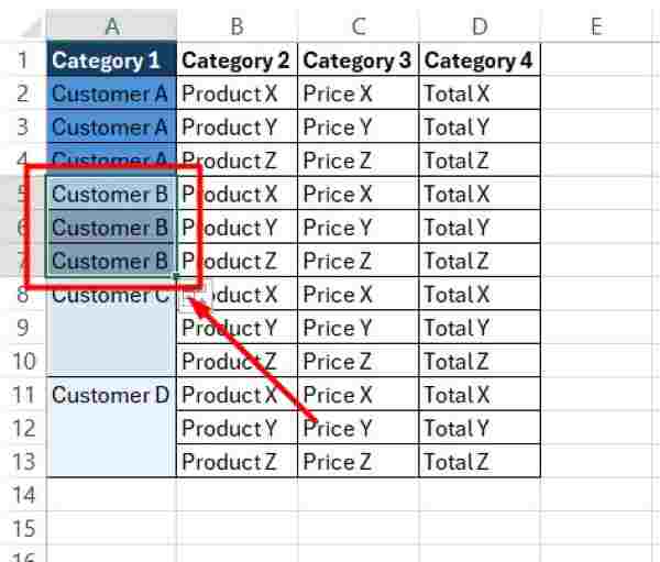
After unmerging the cells, blank spaces will appear. Click on one of these cells and drag its edge to duplicate the data. This action will copy the data from the top cell to the cells below, ensuring consistency.
4. Add Filters to Your Data
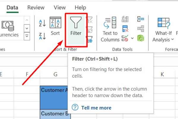
With cells unmerged, apply filters to your data. Click anywhere within the data range, go to the “Data” tab, and click the “Filter” button to add filter arrows to column headers.
5. Filter Your Cell Data
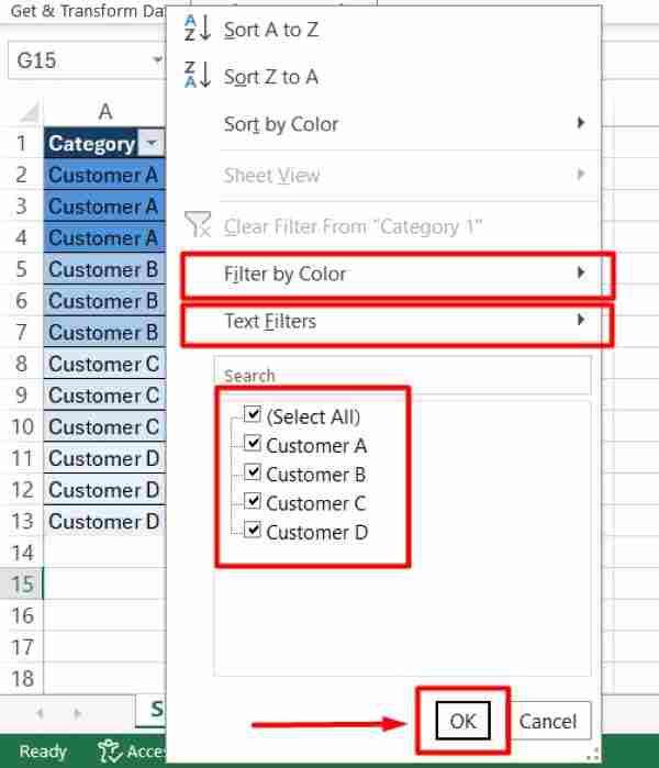
Click the filter arrow in the column header of the data you want to filter.
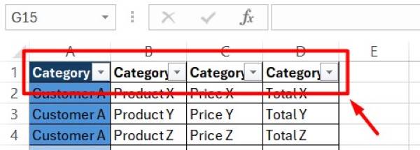
A drop-down menu will appear, allowing you to select specific values or apply text or color filters.
6. Transfer your Filtered Merged Cell Data
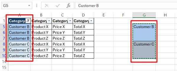
After filtering your data, copy and paste the merged cells that you previously copied from other cells.
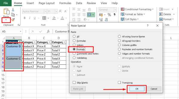
In the Home ribbon, click the “Paste” arrow button and select “Paste Special,” then choose the “format” option. Press “OK” to retain the original format.
We hope you now better understand how to filter merged cells in Excel. If you enjoyed this article, you might also like our article on how to make all merged cells the same size in Excel or our article on how to merge datasets in Excel.

