How to Filter Bold Text in Excel (Easiest Way in 2025)
In this article, we will learn how to filter by bold text in Excel using two different methods: with a custom VBA function and the GET.CELL macro function. Simply follow the steps below.
Filter by Bold Text in Excel
Below are some of the most common methods to easily filter by bold text in Excel.
Method 1: Using a Custom VBA Function
Here is a guide for filtering bold text in Excel with a custom VBA function.
1. Enable Developer Tab
First, open the VBA Editor in Excel to write your custom function for detecting bold text.
In order to open the VBA editor, you must have your “Developer” tab enabled. If you already have the “Developer” tab, you can skip to the next step.
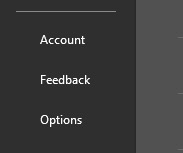
On the Excel ribbon, find and click “File” on the upper left.

Select “Options” found on the lower left after clicking “File”.
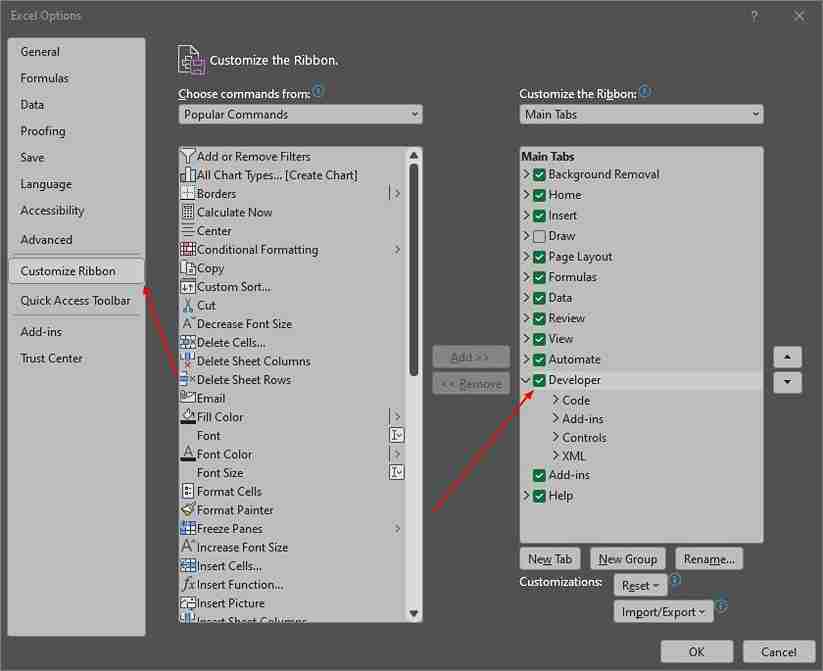
Choose “Customize Ribbon,” and then check the “Developer” option. Click “OK” and it should take you back to your workbook.
2. Open the VBA Editor
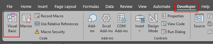
Click the “Developer” tab in the Excel ribbon. Check the “Developer” tab on the upper part of Excel to find the VBA Editor.
Click “Visual Basic” on the “Developer” tab to open the VBA Editor.
2. Insert a New VBA Module
To create a custom function, you need a new VBA module.
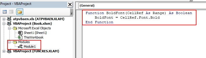
In the VBA Editor, locate your workbook in the “Project Explorer” on the left side.
Right-click the workbook name, select “Insert,” and then choose “Module.” This will create a new module where you can add VBA code.

3. Write the BoldFont Function
Now that you have a module, add the VBA code to create the BoldFont function, which checks if a cell has bold text.
In the new module, type or paste the following code:
| Function BoldFont(CellRef As Range) As Boolean BoldFont = CellRef.Font.Bold End Function |
4. Use the BoldFont Function in Excel
With your function created, return to Excel and apply it to a new column to check if cells contain bold text.
Close the VBA Editor by clicking the “X” at the top-right corner.
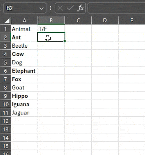
Back in Excel, create a new column next to your data.
In the first cell of the new column, enter the formula =BoldFont(A1), replacing A1 with the reference of the first cell in your data.
Fill down the formula to apply it to the rest of the rows by dragging the small square in the bottom-right corner of the cell or double-clicking it.
5. Filter Data Using the BoldFont Function
After creating a new column that shows whether a row has bold text, use Excel’s built-in filter to display only the rows with bold text.
Click the header of the new column where you applied the BoldFont function.
Click “Data” in the Excel ribbon, then select “Filter.” This adds filter arrows to each column.
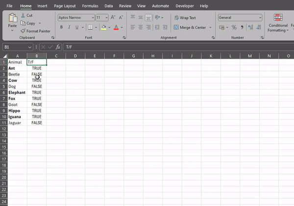
Click the filter arrow on the new column, then deselect “FALSE” to show only rows where BoldFont returned “True”.
6. Save Your Workbook as Macro-Enabled
To keep your VBA code, you must save your workbook in a macro-enabled format.
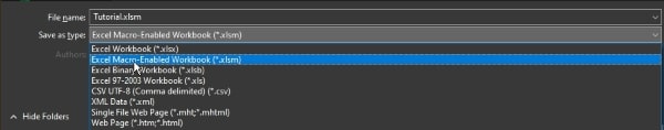
Click “File” in Excel, then select “Save As.”
In the “Save as type” dropdown, select “Excel Macro-Enabled Workbook” (file extension: .xlsm).
Choose where to save your file, give it a name, and click “Save.”
Method 2: Using the GET.CELL Function with Named Ranges
To use the Get.cell function with named ranges to filter bold text in Excel, simply follow these steps.
1. Create a Named Range for GET.CELL
The GET.CELL macro function provides information about cell properties, like font style. To use it, you need to define a named range.
Click “Formulas” in the Excel ribbon.
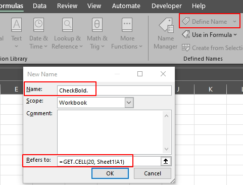
Click “Define Name” to create a new named range.
In the “Name” box, enter a name like “CheckBold.”
In the “Refers to” box, enter:
| =GET.CELL(20, Sheet1!A1) |
Replace Sheet1 with your sheet name and A1 with the starting cell for your data.
Click “OK.”
2. Use the Named Range to Check for Bold Text
With the named range created, use it in Excel to determine if cells contain bold text.
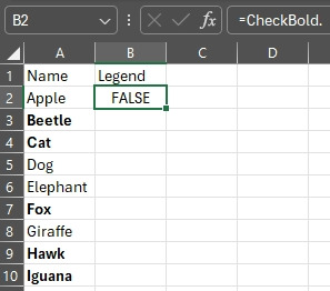
In an empty column, enter =CheckBold.
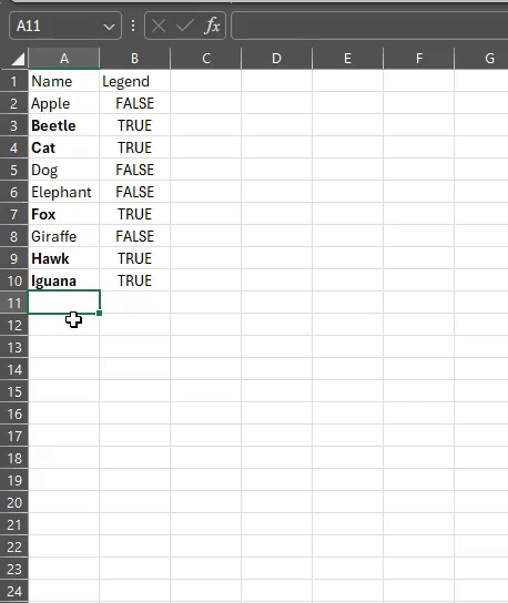
Drag down the formula to apply it to the rest of the rows.
3. Filter Data Using the GET.CELL Function
Once you have the bold status for each row, use Excel’s filter to display only rows with bold text.
Click the header of the column where you used =CheckBold.
Click “Data” in the Excel ribbon, then choose “Filter.”
Click the filter arrow, and deselect “FALSE” to show only rows with bold text.
4. Save Your Workbook
To ensure you don’t lose your work, save your workbook.
Click “File,” then “Save As.”
Select a location, give your file a name, and click “Save.”
We hope you now have a better understanding of how to filter bold text in Excel. If you enjoyed this article, you might also like our article on how to filter by color in Excel or our article on how to use the UNIQUE function in Excel to set up confidence intervals in Google Sheets.