How to Print Frozen Panes in Excel (Easiest Way in 2024)

In this article, we will explore how to print frozen panes on every page in Excel using the Page Setup dialog box. Simply follow the steps below.

How to Print Frozen Panes on Every Page in Excel

Follow the steps below to print frozen panes on every page in Excel using the Page Setup dialog box.

1. Select Rows to Freeze

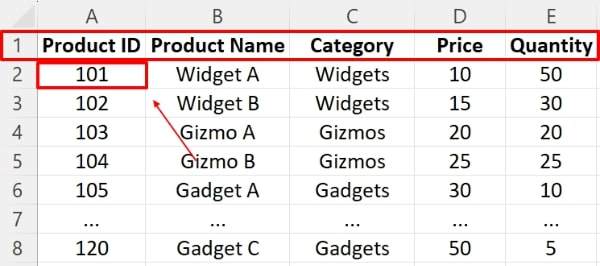
Select the row just below the rows that you want to freeze. For this example, we want to freeze the headers in row 1, so click on cell A2.

2. Freeze Panes

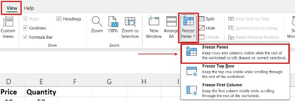
Go to the View tab on the Ribbon. Click Freeze Panes in the Window group, then choose Freeze Panes from the dropdown menu. A solid line will appear below row 1 to indicate that it has been frozen.

3. Access the Page Setup Dialog Box

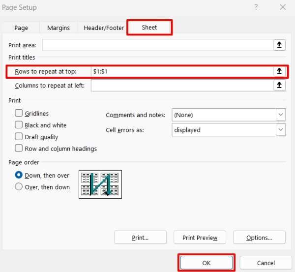
Go to the Page Layout tab on the Ribbon and click on Print Titles. This will open the Page Setup dialog box.

4. Set Print Titles

Go to the Sheet tab. In the Rows to repeat at top box, enter $1:$1 to repeat the first row on every printed page. Click OK.

5. Check Print Preview

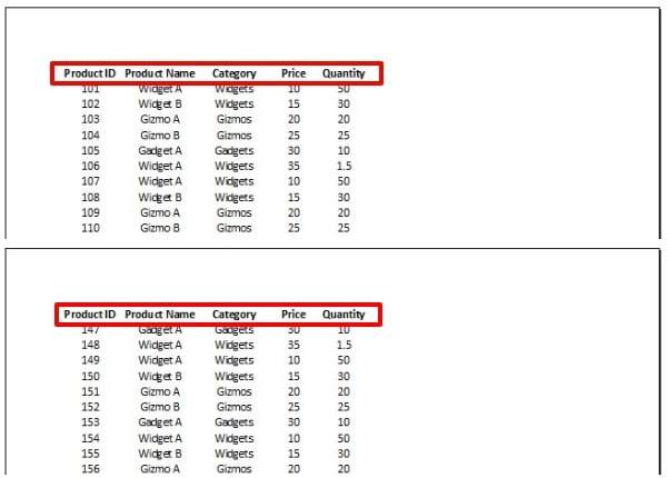
Press Ctrl + P or go to the File tab and select Print. In the Print Preview, you should see the header row repeated at the top of each page. Adjust any other print settings as needed (such as orientation, scaling, margins, etc.) then click Print to print your document.

We hope that you now have a better understanding of how to print frozen panes in Excel. If you enjoyed this article, you might also like our article on how to use rows as print titles in excel and how to print top row on each page in excel.